When we derived a formula for predicting flow rate from pressure dropped by a orifice or venturi tube or, we had to make many assumptions, chief among them being a total lack of friction (i.e. no energy dissipated due to friction) within the moving fluid and perfect stream-line flow (i.e. complete lack of turbulence). Suffice it to say, the flow formulae we have discussed (previous topics) so far are only approximations of reality.
Orifice plates are some of the worst offenders in this regard, since the fluid encounters such abrupt changes in geometry passing through the orifice. Venturi tubes are nearly ideal, since the machined contours of the tube ensure gradual changes in fluid pressure and minimize turbulence.
Read the below article which covers this topic in a more detailed manner for beginners.
However, in the real world we must often do the best we can with imperfect technologies. Orifice plates, despite being less than perfect as flow-sensing elements, are convenient and economical to install in flanged pipes.
Orifice Plates
Orifice plates are also the easiest type of flow element to replace in the event of damage or routine servicing.
In applications such as custody transfer (also called “fiscal” measurement), where the flow of fluid represents product being bought and sold, flow measurement accuracy is paramount.
It is therefore important to figure out how to coax the most accuracy from the common orifice plate in order that we may measure fluid flows both accurately and economically.
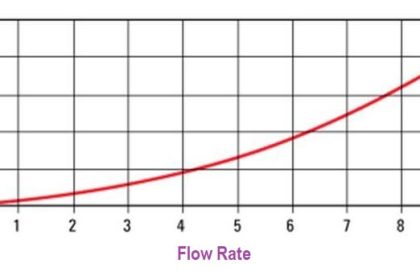
If we compare the true flow rate through a pressure-generating primary sensing element against the theoretical flow rate predicted by an idealized equation, we may notice a substantial discrepancy.
Causes of this discrepancy include, but are not limited to:
- Energy losses due to turbulence and viscosity
- Energy losses due to friction against the pipe and element surfaces
- Unstable location of vena contracta with changes in flow
- Uneven velocity profiles caused by irregularities in the pipe
- Fluid compressibility
- Thermal expansion (or contraction) of the element and piping
- Non-ideal pressure tap location(s)
- Excessive turbulence caused by rough internal pipe surfaces
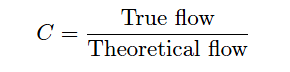
The ratio between true flow rate and theoretical flow rate for any measured amount of differential pressure is known as the discharge coefficient of the flow-sensing element, symbolized by the variable C.
Since a value of 1 represents a theoretical ideal, the actual value of C for any real pressure generating flow element will be less than 1:
For gas and vapor flows, true flow rate deviates even more from the theoretical (ideal) flow value than liquids do, for reasons that have to do with the compressible nature of gases and vapors.
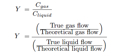
A gas expansion factor (Y ) may be calculated for any flow element by comparing its discharge coefficient for gases against its discharge coefficient for liquids.
As with the discharge coefficient, values of Y for any real pressure-generating element will be less than 1:
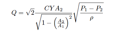
Incorporating these factors into the ideal volumetric flow equation which were discussed in another article (click Here), we arrive at the following formulation:
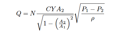
If we wished, we could even add another factor to account for any necessary unit conversions (N), getting rid of the constant √2 in the process:
Sadly, neither the discharge coefficient (C) nor the gas expansion factor (Y ) will remain constant across the entire measurement range of any given flow element.
These variables are subject to some change with flow rate, which further complicates the task of accurately inferring flow rate from differential pressure measurement.
However, if we know the values of C and Y for typical flow conditions, we may achieve good accuracy most of the time.
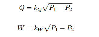
Likewise, the fact that C and Y change with flow places limits on the accuracy obtainable with the “proportionality constant” formulae seen earlier.
Whether we are measuring volumetric or mass flow rate, the k factor calculated at one particular flow condition will not hold constant for all flow conditions:
This means after we have calculated a value for k based on a particular flow condition, we can only trust the results of the equation for flow conditions not too different from the one we used to calculate k.
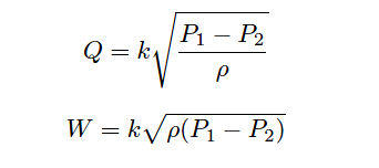
As you can see in both flow equations, the density of the fluid (ρ) is an important factor. If fluid density is relatively stable, we may treat ρ as a constant, incorporating its value into the proportionality factor (k) to make the two formulas even simpler:
However, if fluid density is subject to change over time, we will need some means to continually calculate ρ so our inferred flow measurement will remain accurate. Variable fluid density is a typical state of affairs in gas flow measurement, since all gases are compressible by definition.
A simple change in static gas pressure within the pipe is all that is needed to make ρ change, which in turn affects the relationship between flow rate and differential pressure drop.
The American Gas Association (AGA) provides a formula for calculating volumetric flow of any gas using orifice plates in their #3 Report, compensating for changes in gas pressure and temperature.
A variation of that formula is shown here (consistent with previous formulae in this section):
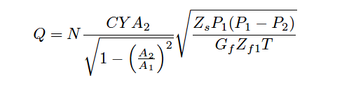
Where,
Q = Volumetric flow rate (SCFM = standard cubic feet per minute)
N = Unit conversion factor
C = Discharge coefficient (accounts for energy losses, Reynolds number corrections, pressure tap locations, etc.)
Y = Gas expansion factor
A1 = Cross-sectional area of mouth
A2 = Cross-sectional area of throat
Zs = Compressibility factor of gas under standard conditions
Zf1 = Compressibility factor of gas under flowing conditions, upstream
Gf = Specific gravity of gas (density compared to ambient air)
T = Absolute temperature of gas
P1 = Upstream pressure (absolute)
P2 = Downstream pressure (absolute)
This equation implies the continuous measurement of absolute gas pressure (P1) and absolute gas temperature (T) inside the pipe, in addition to the differential pressure produced by the orifice plate (P1 − P2).
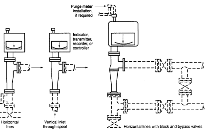
These measurements may be taken by three separate devices, their signals routed to a gas flow computer:
Orifice Flow Meter Compensation

Note the location of the RTD (thermowell), positioned downstream of the orifice plate so the turbulence it generates will not create additional turbulence at the orifice plate.
The American Gas Association (AGA) allows for upstream placement of the thermowell, but only if located at least three feet upstream of a flow conditioner.
In order to best control all the physical parameters necessary for good orifice metering accuracy, it is standard practice for custody transfer flowmeter installations to use honed meter runs rather than standard pipe and pipe fittings.
A “honed run” is a complete piping assembly consisting of a manufactured fitting to hold the orifice plate and sufficient straight lengths of pipe upstream and downstream, the interior surfaces of that pipe machined (“honed”) to have a glass-smooth surface with precise and symmetrical dimensions.
Honed runs ensure minimum disruption to the flowing gas or liquid, thus improving measurement accuracy by avoiding unnecessary turbulence and/or distorted flow profiles. Such piping “runs” are quite expensive, but necessary to achieve flow measurement accuracy worthy of custody transfer.
Orifice Flow Meter
This photograph shows a set of AGA3-compliant orifice meter runs measuring the flow of natural gas:

Note the special transmitter manifolds, built to accept both the differential pressure and absolute pressure (Rosemount model 3051) transmitters.
Also note the quick-change fittings (the ribbed metal housings) holding the orifice plates, to facilitate convenient change-out of the orifice plates which is periodically necessary due to wear. It is not unheard of to replace orifice plates on a daily basis in some industries to ensure the sharp orifice edges necessary for accurate measurement.
Although not visible in this photograph, these meter runs are connected together by a network of shut-off valves directing the flow of natural gas through as few meter runs as desired. When the total gas flow rate is great, all meter runs are placed into service and their respective flow rates summed to yield a total flow measurement.
When the total flow rate decreases, individual meter runs are shut off, resulting in increased flow rates through the remaining meter runs.
This “staging” of meter runs expands the effective turndown or rangeability of the orifice plate as a flow-sensing element, resulting in much more accurate flow measurement over a wide range of flow rates than if a single (large) orifice meter run were used.
Multi-variable Transmitter
An alternative to multiple instruments (differential pressure, absolute pressure, and temperature) installed on each meter run is to use a single multi-variable transmitter capable of measuring gas temperature as well as both static and differential pressures. This approach enjoys the advantage of simpler installation over the multi-instrument approach:

The Rosemount model 3095MV and Yokogawa model EJX910 are examples of multi-variable transmitters designed to perform compensated gas flow measurement, equipped with multiple pressure sensors, a connection port for an RTD temperature sensor, and sufficient digital computing power to continuously calculate flow rate based on the AGA equation.
Such multi-variable transmitters may provide an analog output for computed flow rate, or a digital output where all three primary variables and the computed flow rate may be transmitted to a host system (as shown in the previous illustration).
The Yokogawa EJX910A provides an interesting signal output option: a digital pulse signal, where each pulse represents a specific quantity (either volume or mass) of fluid.
The frequency of this pulse train represents flow rate, while the total number of pulses counted over a period of time represents the total amount of fluid that has passed through the orifice plate over that amount of time.
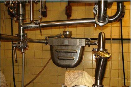
Integral Orifice Plate
This photograph shows a Rosemount 3095MV transmitter used to measure mass flow on a pure oxygen (gas) line. The orifice plate is an “integral” unit immediately below the transmitter body, sandwiched between two flange plates on the copper line.
A three-valve manifold interfaces the model 3095MV transmitter to the integral orifice plate structure:

The temperature-compensation RTD may be clearly seen on the left-hand side of the photograph, installed at the elbow fitting in the copper pipe.
Liquid flow measurement applications may also benefit from compensation, because liquid density changes with temperature. Static pressure is not a concern here, because liquids are considered incompressible for all practical purposes.
Thus, the formula for compensated liquid flow measurement does not include any terms for static pressure, just differential pressure and temperature:

The constant kT shown in the above equation is the proportionality factor for liquid expansion with increasing temperature.
The difference in temperature between the measured condition (T) and the reference condition (Tref ) multiplied by this factor determines how much less dense the liquid is compared to its density at the reference temperature.
It should be noted that some liquids – notably hydrocarbons – have thermal expansion factors significantly greater than water.
This makes temperature compensation for hydrocarbon liquid flow measurement very important if the measurement principle is volumetric rather than mass-based.
If you liked this article, then please subscribe to our YouTube Channel for Instrumentation, Electrical, PLC, and SCADA video tutorials.
You can also follow us on Facebook and Twitter to receive daily updates.
Read Next:
- Orifice Drain and Vent Hole
- DP Transmitter for Level Measurement
- Differential Pressure Level Sensor Errors
- RTD installation after Orifice Plate
- Multi phase Flow Meter Calibration


please send me trmperature compansision formula for dpt flow in dcs
Excelente aplicación favor si pudieran realizar en idioma español
EXCELLENT EXPLANATION FOR SMALL METERING SKID DESIGN .
temperature and pressure compensation for orifice plate is needed when gas flow rate measurmeent.
Koi formula bata sakte ho sir plz
Flow compensation ka