Square-root characteristics of Differential Pressure Flow Meters

As discussed earlier, It should be apparent by now that the relationship between flow rate (whether it be volumetric or mass) and differential pressure for any fluid-accelerating flow element is non-linear: a doubling of flow rate will not result in a doubling of differential pressure.

Rather, a doubling of flow rate will result in a quadrupling of differential pressure. Likewise, a tripling of flow rate results in nine times as much differential pressure developed by the fluid-accelerating flow element.

Differential Pressure Flow Meters

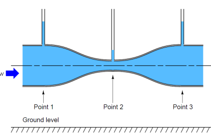
When plotted on a graph, the relationship between flow rate (Q) and differential pressure (ΔP) is quadratic, like one-half of a parabola. Differential pressure developed by a venturi, orifice plate, pitot tube, or any other acceleration-based flow element is proportional to the square of the flow rate:

An unfortunate consequence of this quadratic relationship is that a pressure-sensing instrument connected to such a flow element will not directly sense flow rate. Instead, the pressure instrument will be sensing what is essentially the square of the flow rate.

The instrument may register correctly at the 0% and 100% range points if correctly calibrated for the flow element it connects to, but it will fail to register linearly in between.

Any indicator, recorder, or controller connected to the pressure-sensing instrument will likewise register incorrectly at any point between 0% and 100% of range, because the pressure signal is not a direct representation of flow rate.

In order that we may have indicators, recorders, and controllers that actually do register linearly with flow rate, we must mathematically “condition” or “characterize” the pressure signal sensed by the differential pressure instrument. Since the mathematical function inherent to the flow element is quadratic (square), the proper conditioning for the signal must be the inverse of that: square root.

Just as taking the square-root of the square of a number yields the original number (For positive numbers only!), taking the square-root of the differential pressure signal – which is itself a function of flow squared – yields a signal directly representing flow.

The traditional means of implementing the necessary signal characterization was to install a “square root” function relay between the transmitter and the flow indicator, as shown in the following diagram:

Square-root characteristics of Flow Meters

Note : This is old method & outdated. We are no more using this method in industries.

The modern solution to this problem is to incorporate square-root signal characterization either inside the transmitter or inside the receiving instrument (e.g. indicator, recorder, or controller). Either way, the square-root function must be implemented somewhere in the loop in order that flow may be accurately measured throughout the operating range.

Note :With so many modern instruments being capable of digitally implementing this square-root function, one must be careful to ensure it is only done once in the loop. I have personally witnessed flow-measurement installations where both the pressure transmitter and the indicating device were configured for square-root characterization.

This essentially performed a fourth root characterization on the signal, which is just as bad as no characterization at all! Like anything else technical, the key to successful implementation is a correct understanding of how the system is supposed to work.

Simply memorizing that “the instrument must be set up with square-root to measure flow” and blindly applying that mantra is a recipe for failure.

In the days of pneumatic instrumentation, this square-root function was performed in a separate device called a square-root extractor. The Foxboro model 557 (left) and Moore Products model 65 (right) pneumatic square root extractors are classic examples of this technology:

Note : This is outdated, we are no more dealing with special need of square root extractors in industries. consider this only for learning purpose.

Pneumatic square root extraction relays approximated the square-root function by means of triangulated force or motion. In essence, they were trigonometric function relays, not square-root relays per se.

However, for small angular motions, certain trigonometric functions were close enough to a square-root function that the relays were able to serve their purpose in characterizing the output signal of a pressure sensor to yield a signal representing flow rate.

The following table shows the ideal response of a pneumatic square root relay:

As you can see from the table, the square-root relationship is most evident in comparing the input and output percentage values. For example, at an input signal pressure of 6 PSI (25%), the output signal percentage will be the square root of 25%, which is 50% (0.5 = √0.25) or 9 PSI as a pneumatic signal.

At an input signal pressure of 10 PSI (58.33%), the output signal percentage will be 76.38%, because 0.7638 = √0.5833, yielding an output signal pressure of 12.17 PSI.

When graphed, the function of a square-root extractor is precisely opposite (inverted) of the quadratic function of a flow-sensing element such as an orifice plate, venturi, or pitot tube:

When cascaded – the square-root function placed immediately after the flow element’s “square” function – the result is an output signal that tracks linearly with flow rate (Q). An instrument connected to the square root relay’s signal will therefore register flow rate as it should.

Although analog electronic square-root relays have been built and used in industry for characterizing the output of 4-20 mA electronic transmitters, a far more common implementation of electronic square-root characterization occurs in DP transmitters designed with the square-root function built in.

DP Transmitter Square-root characteristics

This way, no external relay device is necessary to characterize the DP transmitter’s signal into a flow rate signal:

Note : We are using square root extraction function which is available inside the transmitter (software configuration)

Using a characterized DP transmitter, any 4-20 mA sensing instrument connected to the transmitter’s output wires will directly interpret the signal as flow rate rather than as pressure.

A calibration table for such a DP transmitter (with an input range of 0 to 150 inches water column) is shown here:

Once again, we see how the square-root relationship is most evident in comparing the input and output percentages. Note how the percentages in this table precisely match the percentages in the pneumatic relay table: 0% input gives 0% output; 25% input gives 50% output, 50% input gives 70.71% output, etc.

An ingenious solution to the problem of square-root characterization, commonly seen in pneumatic flow-measurement systems where the DP transmitter lacks square-root characterization, is to use an indicating device with a square-root indicating scale.

For example, the following photograph shows a 3-15 PSI “receiver gauge” designed to directly sense the output of a pneumatic DP transmitter:

Note how the gauge mechanism responds directly and linearly to a 3-15 PSI input signal range (note the “3 PSI” and “15 PSI” labels in small print at the extremes of the scale, and the linearly spaced marks around the outside of the scale arc representing 1 PSI each), but how the flow markings (0 through 10 on the inside of the scale arc) are spaced in a non-linear fashion.

An electronic variation on this theme is to draw a square-root scale on the face of a meter movement driven by the 4-20 mA output signal of an electronic DP transmitter:

As with the square-root receiver gauge, the meter movement’s response to the transmitter signal is linear. Note the linear scale (drawn in black text labeled “LINEAR”) on the bottom and the corresponding square-root scale (in green text labeled “FLOW”) on the top. This makes it possible for a human operator to read the scale in terms of (characterized) flow units.

Instead of using complicated mechanisms or circuitry to characterize the transmitter’s signal, a non-linear scale “performs the math” necessary to interpret flow.

A major disadvantage to the use of these non-linear indicator scales is that the transmitter signal itself remains un-characterized. Any other instrument receiving this un-characterized signal will either require its own square-root characterization or simply not interpret the signal in terms of flow at all.

An un-characterized flow signal input to a process controller can cause loop instability at high flow rates, where small changes in actual flow rate result in huge changes in differential pressure sensed by the transmitter.

A fair number of flow control loops operating without characterization have been installed in industrial applications (usually with square-root scales drawn on the face of the indicators, and square-root paper installed in chart recorders), but these loops are notorious for achieving good flow control at only one setpoint value. If the operator raises or lowers the setpoint value, the “gain” of the control loop changes thanks to the nonlinearities of the flow element, resulting in either under-responsive or over-responsive action from the controller.

Despite the limited practicality of non-linear indicating scales, they hold significant value as teaching tools. Closely examine the scales of both the receiver gauge and the 4-20 mA indicating meter, comparing the linear and square-root values at common points on each scale. A couple of examples are highlighted on the electric meter’s scale:

A few correlations between the linear and square-root scales of either the pneumatic receiver gauge or the electric indicating meter verify the fact that the square-root function is encoded in the spacing of the numbers on each instrument’s non-linear scale.

Another valuable lesson we may take from the faces of these indicating instruments is how uncertain the flow measurement becomes at the low end of the scale. Note how for each indicating instrument (both the receiver gauge and the meter movement), the square-root scale is “compressed” at the low end, to the point where it becomes impossible to interpret fine increments of flow at that end of the scale.

At the high end of each scale, it’s a different situation entirely: the numbers are spaced so far apart that it’s easy to read fine distinctions in flow values (e.g. 94% flow versus 95% flow). However, the scale is so crowded at the low end that it’s really impossible to clearly distinguish two different flow values such as 4% from 5%.

This “crowding” is not just an artifact of a visual scale; it is a reflection of a fundamental limitation in measurement certainty with this type of flow measurement. The amount of differential pressure separating different low-range values of flow for a flow element is so little, even small amounts of pressure-measurement error equate to large amounts of flow-measurement error. In other words, it becomes more and more difficult to precisely interpret flow rate as the flow rate decreases toward the low end of the scale.

The “crowding” we see on these indicator’s square-root scales is a visual reflection of this fundamental problem: even a small error in interpreting the pointer’s position at the low end of the scale can yield major errors in flow interpretation.

A technical term used to quantify this problem is turndown. “Turndown” refers to the ratio of high-range measurement to low-range measurement possible for an instrument while maintaining reasonable accuracy. For pressure-based flowmeters, which must deal with the non-linearities of Bernoulli’s Equation, the practical turndown is often no more than 3 to 1 (3:1).

This means a flowmeter ranged for 0 to 300 GPM might only read with reasonable accurately down to a flow of 100 GPM. Below that, the accuracy becomes so poor that the measurement is almost useless. Advances in DP transmitter technology have pushed this ratio further, perhaps as far as 10:1 for certain installations.

However, the fundamental problem is not transmitter resolution, but rather the non-linearity of the flow element itself. This means any source of pressure-measurement error – whether originating in the transmitter’s pressure sensor or not – compromises our ability to accurately measure flow at low rates.

Even with a perfectly calibrated transmitter, errors resulting from wear of the flow element (e.g. a dulled edge on an orifice plate) or from uneven liquid columns in the impulse tubes connecting the transmitter to the element, will cause large flow-measurement errors at the low end of the instrument’s range where the flow element produces only small differential pressures.

Everyone involved with the technical details of flow measurement needs to understand this fact: the fundamental problem of limited turndown is grounded in the physics of turbulent flow and potential/kinetic energy exchange for these flow elements.

Technological improvements will help, but they cannot overcome the limitations imposed by physics. If better turndown is required for a particular flow-measurement application, an entirely different flowmeter technology should be considered.

If you liked this article, then please subscribe to our YouTube Channel for Electrical, Electronics, Instrumentation, PLC, and SCADA video tutorials.

You can also follow us on Facebook and Twitter to receive daily updates.

Read Next:

• Turbine Flow Meter Installation
• Insertion Flow Meter Principle
• Variable Area Flow Meters
• Flow Sensors Questions
• DP Transmitter Level Sensors