The Mean time between failures (MTBF) of any system dependent upon certain critical components may be extended by duplicating those components in parallel fashion, such that the failure of only one does not compromise the system as a whole. This is called redundancy.
A common example of component redundancy in instrumentation and control systems is the redundancy offered by distributed control systems (DCS), where processors, network cables, and even I/O (input/output) channels may be equipped with “hot standby” duplicates ready to assume functionality in the event the primary component fails.
Redundancy tends to extend the MTBF of a system without necessarily extending its service life. A DCS, for example, equipped with redundant microprocessor control modules in its rack, will exhibit a greater MTBF because a random microprocessor fault will be covered by the presence of the spare (“hot standby”) microprocessor module.
However, given the fact that both microprocessors are continually powered, and therefore tend to “wear” at the same rate, their operating lives will not be additive. In other words, two microprocessors will not function twice as long before wear-out than one microprocessor.
The extension of MTBF resulting from redundancy holds true only if the random failures are truly independent events – that is, not associated by a common cause.
To use the example of a DCS rack with redundant microprocessor control modules again, the susceptibility of that rack to a random microprocessor fault will be reduced by the presence of redundant microprocessors only if the faults in question are unrelated to each other, affecting the two microprocessors separately.
There may exist common-cause fault mechanisms capable of disabling both microprocessor modules as easily as it could disable one, in which case the redundancy adds no value at all.
Examples of such common-cause faults include power surges (because a surge strong enough to kill one module will likely kill the other at the same time) and a computer virus infection (because a virus able to attack one will be able to attack the other just as easily, and at the same time).
Redundancy in Control Systems
A simple example of component redundancy in an industrial instrumentation system is dual DC power supplies feeding through a diode module.
The following photograph shows a typical example, in this case a pair of Allen-Bradley AC-to-DC power supplies for a DeviceNet digital network:

If either of the two AC-to-DC power supplies happens to fail with a low output voltage, the other power supply is able to carry the load by passing its power through the diode redundancy module:

This redundancy module has its own MTBF value, and so by including it in the system we are adding one more component that can fail.
However, the MTBF rate of a simple diode network greatly exceeds that of an entire AC-to- DC power supply, and so we find ourselves at a greater level of reliability using this diode redundancy module than if we did not (and only had one power supply).
In order for redundant components to actually increase system MTBF, the potential for common cause failures must be addressed. For example, consider the effects of powering redundant AC-to- DC power supplies from the exact same AC line.
Redundant power supplies would increase system reliability in the face of a random power supply failure, but this redundancy would do nothing at all to improve system reliability in the event of the common AC power line failing! In order to enjoy the fullest benefit of redundancy in this example, we must source each AC-to-DC power supply from a different (unrelated) AC line.
Another example of redundancy in industrial instrumentation is the use of multiple transmitters to sense the same process variable, the notion being that the critical process variable will still be monitored even in the event of a transmitter failure. Thus, installing redundant transmitters should increase the MTBF of the system’s sensing ability.
Here again, we must address common-cause failures in order to reap the full benefits of redundancy. If three liquid level transmitters are installed to measure the exact same liquid level, their combined signals represent an increase in measurement system MTBF only for independent faults.
A failure mechanism common to all three transmitters will leave the system just as vulnerable to random failure as a single transmitter. In order to achieve optimum MTBF in redundant sensor arrays, the sensors must be immune to common faults.
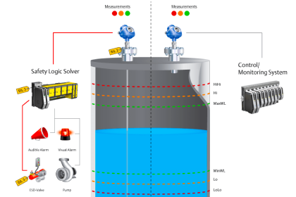
Level Transmitter Voting System
In this example, three different types of level transmitter monitor the level of liquid inside a vessel, their signals processed by a selector function programmed inside a DCS:

Here, level transmitter 23a is a guided-wave radar (GWR), level transmitter 23b is a tape-and float, and level transmitter 23c is a differential pressure sensor. All three level transmitters sense liquid level using different technologies, each one with its own strengths and weaknesses.
Better redundancy of measurement is obtained this way, since no single process condition or other random event is likely to fault more than one of the transmitters at any given time.
For instance, if the process liquid density happened to suddenly change, it would affect the measurement accuracy of the differential pressure transmitter (LT-23c), but not the radar transmitter nor the tape-and-float transmitter.
If the process vapor density were to suddenly change, it might affect the radar transmitter (since vapor density generally affects dielectric constant, and dielectric constant affects the propagation velocity of electromagnetic waves, which in turn will affect the time taken for the radar pulse to strike the liquid surface and return), but this will not affect the float transmitter’s accuracy nor will it affect the differential pressure transmitter’s accuracy.
Surface turbulence of the liquid inside the vessel may severely affect the float transmitter’s ability to accurately sense liquid level, but it will have little effect on the differential pressure transmitter’s reading nor the radar transmitter’s measurement (assuming the radar transmitter is shrouded in a stilling well.
If the selector function takes either the median (middle) measurement or an average of the best 2-out-of-3 (“2oo3”), none of these random process occurrences will greatly affect the selected measurement of liquid level inside the vessel.
True redundancy is achieved here since the three-level transmitters are not only less likely to (all) fail simultaneously than for any single transmitter to fail, but also because the level is being sensed in three completely different ways.
A crucial requirement for redundancy to be effective is that all redundant components must have precisely the same process function. In the case of redundant DCS components such as processors, I/O cards, and network cables, each of these redundant components must do nothing more than serve as “backup” spares for their primary counterparts.
If a particular DCS node were equipped with two processors – one as the primary and another as a secondary (backup) – but yet the backup processor were tasked with some detail specific to it and not to the primary processor (or vice-versa), the two processors would not be truly redundant to each other.
If one processor were to fail, the other would not perform exactly the same function, and so the system’s operation would be affected (even if only in a small way) by the processor failure.
Likewise, redundant sensors must perform the exact same process measurement function in order to be truly redundant. A process equipped with triplicate measurement transmitters such as the previous example were a vessel’s liquid level was being measured by a guided-wave radar, tape-and-float, and differential pressure based level transmitters, would enjoy the protection of redundancy if and only if all three transmitters sensed the exact same liquid level over the exact same calibrated range.
This often represents a challenge, in finding suitable locations on the process vessel for three different instruments to sense the exact same process variable.
Quite often, the pipe fittings penetrating the vessel (often called nozzles) are not conveniently located to accept multiple instruments at the points necessary to ensure consistency of measurement between them. This is often the case when an existing process vessel is retrofitted with redundant process transmitters.
New construction is usually less of a problem, since the necessary nozzles and other accessories may be placed in their proper positions during the design stage.
If fluid flow conditions inside a process vessel are excessively turbulent, multiple sensors installed to measure the same variable will sometimes report significant differences.
Multiple temperature transmitters located in close proximity to each other on a distillation column, for example, may report significant differences of temperature if their respective sensing elements (thermocouples, RTDs) contact the process liquid or vapor at points where the flow patterns vary.
Multiple liquid level sensors, even of the same technology, may report differences in liquid level if the liquid inside the vessel swirls or “funnels” as it enters and exits the vessel.
Not only will substantial measurement differences between redundant transmitters compromise their ability to function as “backup” devices in the event of a failure, but such differences may also actually “fool” a redundant system into thinking one or more of the transmitters has already failed, thereby causing the deviating measurement to be ignored.
To use the triplicate level-sensing array as an example again, suppose the radar-based level transmitter happened to register two inches greater level than the other two transmitters due to the effects of liquid swirl inside the vessel.
If the selector function is programmed to ignore such deviating measurements, the system degrades to a duplicate-redundant instead of triplicate-redundant array.
In the event of a dangerously low liquid level, for example, only the radar-based and float-based level transmitters will be ready to signal this dangerous process condition to the control system, because the pressure-based level transmitter is registering too high.