Calibration refers to the adjustment of an instrument so its output accurately corresponds to its input throughout a specified range.
The only way we can know that an instrument’s output accurately corresponds to its input over a continuous range is to subject that instrument to known input values while measuring the corresponding output signal values. This means we must use trusted standards to establish known input conditions and to measure output signals.
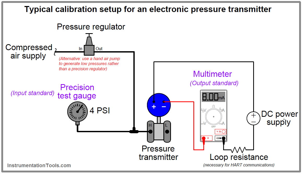
The following examples show both input and output standards used in the calibration of pressure and temperature transmitters:
A noteworthy exception is the case of digital instruments, which output digital rather than analog signals. In this case, there is no need to compare the digital output signal against a standard, as digital numbers are not liable to calibration drift.
However, the calibration of a digital instrument still requires comparison against a trusted standard in order to validate an analog quantity.
For example, a digital pressure transmitter must still have its input calibration values validated by a pressure standard, even if the transmitter’s digital output signal cannot drift or be misinterpreted.
It is the purpose of this section to describe procedures for efficiently calibrating different types of instruments.
Linear Instruments
The simplest calibration procedure for an analog, linear instrument is the so-called zero-and-span method. The method is as follows:
- Apply the lower-range value stimulus to the instrument, wait for it to stabilize
- Move the “zero” adjustment until the instrument registers accurately at this point
- Apply the upper-range value stimulus to the instrument, wait for it to stabilize
- Move the “span” adjustment until the instrument registers accurately at this point
- Repeat steps 1 through 4 as necessary to achieve good accuracy at both ends of the range
An improvement over this crude procedure is to check the instrument’s response at several points between the lower- and upper-range values. A common example of this is the so-called five-point calibration where the instrument is checked at 0% (LRV), 25%, 50%, 75%, and 100% (URV) of range.
A variation on this theme is to check at the five points of 10%, 25%, 50%, 75%, and 90%, while still making zero and span adjustments at 0% and 100%. Regardless of the specific percentage points chosen for checking, the goal is to ensure that we achieve (at least) the minimum necessary accuracy at all points along the scale, so the instrument’s response may be trusted when placed into service.
Yet another improvement over the basic five-point test is to check the instrument’s response at five calibration points decreasing as well as increasing. Such tests are often referred to as Up-down calibrations. The purpose of such a test is to determine if the instrument has any significant hysteresis: a lack of responsiveness to a change in direction.
Some analog instruments provide a means to adjust linearity. This adjustment should be moved only if absolutely necessary! Quite often, these linearity adjustments are very sensitive, and prone to over-adjustment by zealous fingers.
The linearity adjustment of an instrument should be changed only if the required accuracy cannot be achieved across the full range of the instrument. Otherwise, it is advisable to adjust the zero and span controls to “split” the error between the highest and lowest points on the scale, and leave linearity alone.
The procedure for calibrating a “smart” digital transmitter – also known as trimming – is a bit different. Unlike the zero and span adjustments of an analog instrument, the “low” and “high” trim functions of a digital instrument are typically non-interactive.
This means you should only have to apply the low- and high-level stimuli once during a calibration procedure. Trimming the sensor of a “smart” instrument consists of these four general steps:
- Apply the lower-range value stimulus to the instrument, wait for it to stabilize
- Execute the “low” sensor trim function
- Apply the upper-range value stimulus to the instrument, wait for it to stabilize
- Execute the “high” sensor trim function
Likewise, trimming the output (Digital-to-Analog Converter, or DAC) of a “smart” instrument consists of these six general steps:
- Execute the “low” output trim test function
- Measure the output signal with a precision milliammeter, noting the value after it stabilizes
- Enter this measured current value when prompted by the instrument
- Execute the “high” output trim test function
- Measure the output signal with a precision milliammeter, noting the value after it stabilizes
- Enter this measured current value when prompted by the instrument
After both the input and output (ADC and DAC) of a smart transmitter have been trimmed (i.e. calibrated against standard references known to be accurate), the lower- and upper-range values may be set.
In fact, once the trim procedures are complete, the transmitter may be ranged and ranged again as many times as desired. The only reason for re-trimming a smart transmitter is to ensure accuracy over long periods of time where the sensor and/or the converter circuitry may have drifted out of acceptable limits.
This stands in stark contrast to analog transmitter technology, where re-ranging necessitates re-calibration every time.
Non-linear Instruments
The calibration of inherently nonlinear instruments is much more challenging than for linear instruments. No longer are two adjustments (zero and span) sufficient, because more than two points are necessary to define a curve.
Examples of nonlinear instruments include expanded-scale electrical meters, square root characterizers, and position-characterized control valves.
Every nonlinear instrument will have its own recommended calibration procedure, so I will defer you to the manufacturer’s literature for your specific instrument. I will, however, offer one piece of advice: when calibrating a nonlinear instrument, document all the adjustments you make (e.g. how many turns on each calibration screw) just in case you find the need to “re-set” the instrument back to its original condition.
More than once I have struggled to calibrate a nonlinear instrument only to find myself further away from good calibration than where I originally started. In times like these, it is good to know you can always reverse your steps and start over!
Discrete Instruments
The word “discrete” means individual or distinct. In engineering, a “discrete” variable or measurement refers to a true-or-false condition. Thus, a discrete sensor is one that is only able to indicate whether the measured variable is above or below a specified setpoint.
Examples of discrete instruments are process switches designed to turn on and off at certain values. A pressure switch, for example, used to turn an air compressor on if the air pressure ever falls below 85 PSI, is an example of a discrete instrument.
Discrete instruments require periodic calibration just like continuous instruments. Most discrete instruments have just one calibration adjustment: the set-point or trip-point. Some process switches have two adjustments: the set-point as well as a deadband adjustment.
The purpose of a deadband adjustment is to provide an adjustable buffer range that must be traversed before the switch changes state. To use our 85 PSI low air pressure switch as an example, the set-point would be 85 PSI, but if the deadband were 5 PSI it would mean the switch would not change state until the pressure rose above 90 PSI (85 PSI + 5 PSI).
When calibrating a discrete instrument, you must be sure to check the accuracy of the set-point in the proper direction of stimulus change. For our air pressure switch example, this would mean checking to see that the switch changes states at 85 PSI falling, not 85 PSI rising.
If it were not for the existence of deadband, it would not matter which way the applied pressure changed during the calibration test. However, deadband will always be present in a discrete instrument, whether that deadband is adjustable or not.
For example, a pressure switch with a deadband of 5 PSI set to trip at 85 PSI falling would re-set at 90 PSI rising. Conversely, a pressure switch (with the same deadband of 5 PSI) set to trip at 85 PSI rising would re-set at 80 PSI falling.
In both cases, the switch “trips” at 85 PSI, but the direction of pressure change specified for that trip point defines which side of 85 PSI the re-set pressure will be found.
A procedure to efficiently calibrate a discrete instrument without too many trial-and-error attempts is to set the stimulus at the desired value (e.g. 85 PSI for our hypothetical low-pressure switch) and then move the set-point adjustment in the opposite direction as the intended direction of the stimulus (in this case, increasing the set-point value until the switch changes states).
The basis for this technique is the realization that most comparison mechanisms cannot tell the difference between a rising process variable and a falling setpoint (or vice-versa).
Thus, a falling pressure may be simulated by a rising set-point adjustment. You should still perform an actual changing-stimulus test to ensure the instrument responds properly under realistic circumstances, but this “trick” will help you achieve good calibration in less time.
Also Read : SMART Transmitter Calibration