In PID tuning, it is required every time that the process variable is maintained around the set variable without affecting the process. But what happens if the process variable, which is derived from real-time feedback, is delayed every time by a few seconds?
Then there will be a big time deviation in the process control, and the variable will not be maintained around the set point. Such delays in PID are called the dead time. In this post, we will see the concept of dead time compensation in PID tuning.
Why is dead time important in PID tuning?
Let us understand this with a very simple example of an electric heater, which has a temperature sensor to sense the heating temperature. When the PID increases the heater power, the heater starts heating immediately, but the sensor shows the temperature rise only after 10 seconds. 5 seconds have passed, but still there is no feedback on the temperature, so the heater will continue to increase its power, thinking that the temperature is still low.
After 10 seconds, when the feedback comes, the temperature has already become so high above the set point that the PID will immediately start to decrease the output in an abrupt manner and create an oscillatory behaviour. This dead time of 10 seconds on average, which was caused by the sensor giving feedback a little late, is harmful to the process. That is why dead time is very important to understand in PID tuning.
What is dead time compensation in PID?
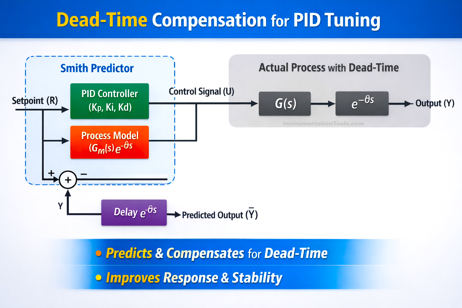
As the name implies, the concept is to compensate for dead time by prediction. So here, if the heater power increases by 20%, then the model instantly predicts that the temperature will increase by 3 degrees Celsius after the delay. So, the PID will not wait for the real feedback, and instead, it will act based on this prediction. Due to this, the PID will start to maintain the power from that point only, and the system remains stable. This concept is also called the Smith Predictor concept, and is termed finally as dead time compensation.
But here comes a major correction. The model not only predicts but also takes real-time feedback for correct output. This forms a smart loop that reacts fast and stays accurate. Let us understand clearly how the model works.
When the PID loop starts, the internal process model immediately begins predicting how the temperature will rise in the next few seconds. Every scan (say every 1 second), this predicted value is used as the temporary feedback for the PID instead of the real sensor. At the same time, each predicted value is pushed into a FIFO buffer whose length equals the dead time (10 seconds = 10 samples). This buffer represents the “virtual sensor delay.” After 10 seconds, the first real temperature measurement arrives from the actual sensor.
The Smith Predictor then compares this real value with the predicted value that was generated 10 seconds earlier (the oldest value sitting in the buffer). If there is a mismatch, the error is applied to correct the internal model so that future predictions become more accurate.
After correction, the PID continues to operate on the model’s current predicted process output, not on the delayed measurement. Once this comparison and correction are done, the loop repeats: every second, the model predicts the next temperature, pushes it into the buffer, uses the newest prediction for PID control, and pulls out the oldest prediction to compare with the newest real sensor reading.
Standard PID blocks in PLC’s do not include dead time compensation, as it is very advanced. Some PLC vendors either include that as an optional library or add-on, but these are not free and often require licenses. It is mostly used in DCS, thus. This is because dead time varies a lot, requires a process model, requires more PLC memory with higher performance CPUs, and is not needed for everyday fast loops. But you can customize this logic as per your requirement in the PLC program on a small scale basis.
Programming Steps for Implementing Dead-Time Compensation (Smith Predictor)
To implement dead-time compensation in a PLC, the first step is to build an internal process model, which simply means a mathematical copy of your real plant inside the PLC program. For example, if increasing a heater output by 10% normally causes the temperature to rise slowly with a time constant of 40 seconds and a dead time of 10 seconds, you create a small formula or block in the PLC that behaves the same way: a process gain block, a first-order lag block, and a dead-time buffer.
This model receives the PID output every scan and produces an estimated process value, and this is the “predicted temperature” the PID will use as feedback. Next, you implement a FIFO buffer whose size equals dead time ÷ scan time (e.g., 10 seconds dead time at 1-second scan needs 10 samples). Every predicted PV is pushed into this buffer to simulate how the real sensor would behave after the delay.
The real sensor PV is also read continuously. When the real PV arrives for the same point in time, you compare the real PV with the model’s oldest buffer value; any difference is used to correct the model’s output to avoid drift. After correction, the PID continues running on the model PV, new predictions are generated each cycle, the buffer shifts by one position, and the entire prediction–correction loop repeats every scan. This way, the PID always “sees the future” instead of waiting for delayed feedback, while the real PV is used in the background to keep the model accurate.
Smith Predictor functionality is not commonly built into basic PLC PID instructions, but it is widely available in advanced process controllers and DCS platforms. In ABB (800xA), Emerson DeltaV, Yokogawa CENTUM VP, Honeywell Experion PKS, and Siemens PCS7/APC packages, dead-time compensation is available as a standard or optional advanced control function block.
In Schneider EcoStruxure Process Expert and Rockwell PlantPAx (via PIDE + APC templates), preconfigured modules or add-on instructions exist for model-based prediction and dead-time handling. Some PACs, like Beckhoff TwinCAT and B&R Automation Studio, offer model-based control libraries where a Smith Predictor block is already included.
At the instrumentation level, certain specialty temperature controllers (Eurotherm, Omron advanced models, and ABB single-loop controllers) include dead-time compensation as a menu-based feature. In most standard PLCs (Allen-Bradley CompactLogix/ControlLogix, Siemens S7-1200/1500 ladder/STL environments), you typically must implement the buffer, model, and correction logic manually, because the default PID block does not contain a Smith Predictor.