Proportional Controller Principle

If the outflow (Qo) increases then the level in the tank will fall. The pressure sensed by the level transmitter, which is representative of the level in the tank, will also fall causing a decrease in the output signal from the level transmitter. This output signal is fed to the (air to close) control valve (valve fully open with 20 kPa signal, fully closed with 100 kPa signal). A falling level will therefore cause the valve to progressively open and hence raise the level in the tank. The system as shown is somewhat impractical as the initial setpoint conditions will need to be set by some manual method and then ensuring that steady state conditions are achieved with the valve at, say 50% opening and a level transmitter output of 60 kPa (50% range).

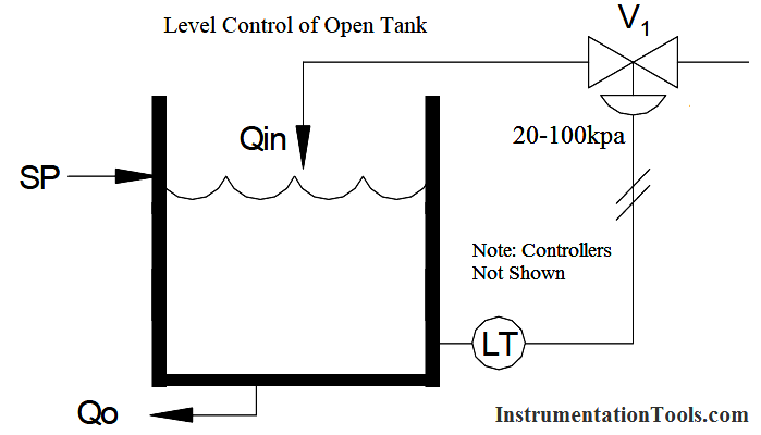
This simple system does illustrate however a major disadvantage with proportional control. Notice that the control signal (valve opening) can only change when the level signal is changing. Thus if a disturbance occurs, say an increase in demand, the level will drop and the output from the level transmitter will also fall. This will cause the air to close valve to open more, hence increasing the inflow.

After a period of time the inflow will have increased such that a now mass balance is established between inflow and outflow. But where is the level at this time?

Certainly not at the setpoint. In the example given it will stabilize at some steady state level below the setpoint. This steady state deviation is known as offset and is inherent in all proportional control systems. Despite this obvious disadvantage, (we cannot return the process to the setpoint after a disturbance with proportional control) this mode of control will form the basis for all our control strategies. In the next section we will discuss a more practical control scheme using proportional control and also ways of lessening the problem of offset.

Example 1

A tank has inflow and outflow equal to 50% of maximum and its level is at the setpoint, say 50%. A step change in outflow occurs to 60% (+10%). Outflow now exceeds inflow so the level will fall. The output from the level transmitter will also fall and, for our system, will match the fall in level – say 1% change in signal for a 1% change in level. The LT signal will open the A/C valve more, by 1% in fact. The inflow is now 51%, still less than the outflow. The level will continue to fall until inflow equals outflow, i.e., (60%). This can only happen when the LT signal has changed by 10%) and this change reflects a drop in level on 10%: i.e., 10% offset.

To restore the process to the setpoint requires a further increase of inflow. This increase can only be achieved by a further decrease in signal to the valve (i.e., as decrease in LT output corresponding to a further decrease in level).

With the conditions as stated in the example there is no way in which a 50% level can be achieved with a 60% outflow. A 50% level with a 60% outflow requires a 60% inflow. Our systems can only provide a 60% inflow from a 40% level signal.

Example 2

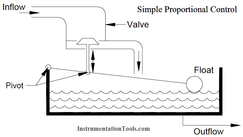
An alternative method of illustrating proportional control is by means of a simple float system (Below Figure). Assume the inflow and outflow are equal and the level is at the setpoint. If an increase in outflow occurs the level in the tank must fall. The float will also fall as the level falls. This drop in float position will cause the valve on the inflow to open more thus increasing the inflow. Eventually the fall in level will result in a valve opening, which will restore the mass balance between the inflow and the outflow.

Note an increased inflow can only be achieved as a result of a lower level in the tank. The level is no longer at the setpoint an offset has been generated.

Summary:

• Proportional control provides a control signal, proportional to the magnitude and direction of the error signal.
• After a disturbance, proportional control will provide only a new mass balance situation. A change in control signal requires a change in error signal, therefore offset will occur.
• Proportional control stabilizes an error; it does not remove it.

Proportional Control Terminology

M = Measurement Signal
SP = Setpoint
e = Error

e = SP –- M

Note:

If M>SP then e is negative
If M<SP then e is positive

m = Controller Signal Output

Δ in O/P = final –- initial

k = Gain

when controller uses e = SP -– M
THEN K is negative for Direct Acting
K is positive for Reverse Acting

b = bias (usually 50% of output span)

m = ke + b

↑↑ Direct Action M↑m↑
↑↓ Reverse Action M↑m↓

PB = Proportional Band

Small (narrow) PB = High Gain
Large (wide) PB = Low Gain

Practical Proportional Control

A more practical proportional control scheme can be achieved by inserting a controller between the level transmitter and the control valve.In our example of an open tank with a valve on the inflow it would be reasonable to assume that the valve should close in the event of an air supply failure to prevent the tank overflowing, i.e., an air to open valve.

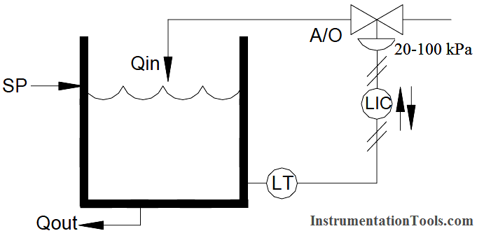
To achieve the necessary control action on, say, a falling tank level it is necessary to convert the decreasing output of the level transmitter to an increasing input signal to the control valve. The level controller will perform this function and is termed an indirect or reverse acting (↑↓) controller. It can be seen that if the valve action had been chosen air to close, then this reversal would not have been required and a direct (↑↑) acting controller could have been used. Normally controllers are capable of performing either control action, direct or reverse, by a simple switching process.

The controller will also accept our desired setpoint input and perform the comparison between setpoint and measurement to calculate the error’s magnitude and direction.

Up to now we have only assumed proportionality constant or one, i.e., the control signal equals the input error. Is this always the best ratio? Consider the following graphs of input, output and level with respect to time:

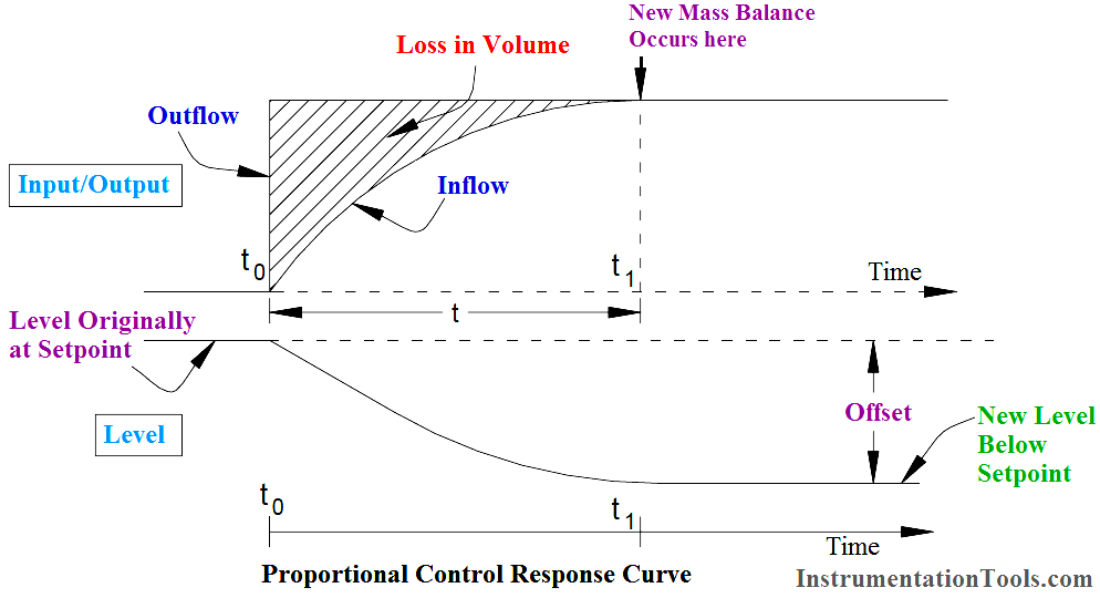
It can be seen that a step increase in demand (outflow) has occurred at time “t0”. the resulting control correction has caused a new mass balance to be achieved after some time t1. At this time, under the new mass balance conditions, the level will stabilize at some level below the original setpoint, i.e., an offset has occurred, the loss in volume being represented by the shaded area between the input and output curves.

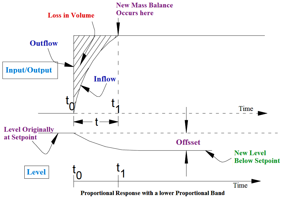
Consider now the same demand disturbance but with the control signal increased in relative magnitude with respect to the error signal; i.e.,instead of control signal = error signal, control signal = error signal x gain constant (k). Clearly for any given error signal the control signal will be increased in magnitude, the inflow will be increased, and a new mass balance will be achieved in a shorter time as shown in Above Figure. (If we refer back to our simple ballcock system in section 3.3, it can be seen that the gain could be varied by adjusting the position of the valve operating link on the float arm.) The offset is much reduced. In instrumentation this adjustment of controller gain is referred to as proportional band (PB).

Proportional band is defined as that input signal span change, in percent, which will cause a hundred percent change in output signal.

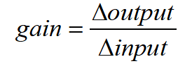
For example if an input signal span change of 100% is required to give an output change of 100% the system is said to have a proportional band of 100%. If the system was now adjusted such that the 100% change in output was achieved with only a 50% change in input signal span then the proportional band is now said to be 50%. There is a clear relationship between proportional band and gain. Gain can be defined as the ratio between change in output and change in input.

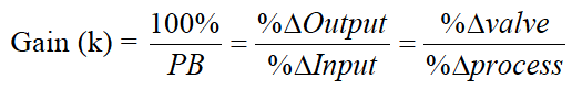
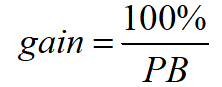
By inspection it can be seen that a PB of 100% is the same as a gain of one since change of input equals change in output. PB is the reciprocal of gain, expressed as a percentage. The general relationship is:

Example:

What is the gain of a controller with a PB of? a) 40%, b) 200%

Gain = 100% / P.B = 100/40 = 2.5

Gain = 100% / P.B = 100/200 = 0.5

What will the PB setting in percent for a controller with gain of? a) 3, b) 0.4

P.B = 100%/Gain = 100/3 = 33.33%

P.B = 100%/Gain = 100/0.4 = 250%

Small values of PB (high gain) are usually referred to as narrow proportional band whilst low gain is termed wide proportional band. Note there is no magic figure to define narrow or wide proportional band, relative values only are applicable, for example, 15% PB is wider than 10% PB, 150% PB is narrower than 200% PB.

We have seen from the two earlier examples that increasing the gain, (narrowing the PB) caused the offset to be decreased. Can this procedure be used to reduce the offset to zero?

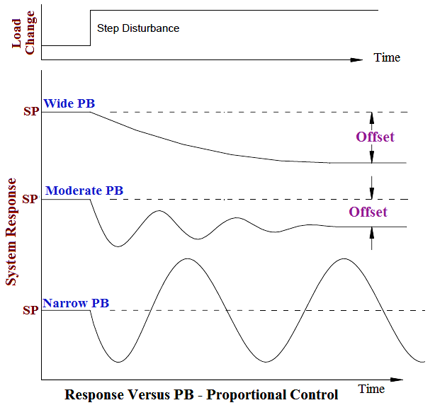
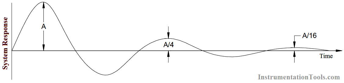
Fig : ¼ Decay Response Curve

With reference to Response Vs PB Figure , consider a high gain system (say gain = 50, PB = 2%). Under steady state conditions with the process at the setpoint the inflow will have a constant value. This is usually taken to be a control signal of 50% for a proportional controller with the process at the setpoint. In other words we have a 50% control capability. With our high gain system it can be seen that the maximum control signal will be achieved with an error of =1% (control signal = gain x error). This control signal will cause the valve to go fully open, the level will rise and the process will cross the setpoint. The error signal will now change sign and when the error again exceeds 1% the resultant control signal will now cause the valve to fully close hence completely stopping the inflow. This process will be repeated continuously – we have reverted to an on/off control situation with all the disadvantages previously mentioned. Obviously there must be some optimum setting of PB which is a trade off between the highly stable but sluggish low gain system with large offset, and the fast acting, unstable on/off system with mean offset equal to zero. The accepted optimum setting is one that causes the process to decay in a ¼ decay method as shown in Above Figures.

The quarter decay curves show that the process returns to a steady state condition after three cycles of damped oscillation. This optimization will be discussed more fully in the section on controller tuning.

Recall the output of a proportional controller is equal to:

m = ke

where m = control signal

Clearly if the error is zero the control signal will be zero, this is an undesirable situation. Therefore for proportional control a constant term or bias must be added to provide a steady state control signal when the error is zero.

For the purposes of this course we will assume the steady state output of a proportional controller when at the setpoint to be 50%. The equation for proportional control becomes:

m = ke + b

where b = bias

Summary

• The controller action must be chosen (either direct ↑↑ or reverse ↑↓ ) to achieve the correct control response.
• Proportional Band =100%/gain or gain = 100%/PB
• The optimum settings for PB should result in the process decaying in a ¼ decay mode.