Inst ToolsInst ToolsInst Tools
  • Courses
  • Automation
    • PLC
    • Control System
    • Safety System
    • Communication
    • Fire & Gas System
  • Instrumentation
    • Design
    • Pressure
    • Temperature
    • Flow
    • Level
    • Vibration
    • Analyzer
    • Control Valve
    • Switch
    • Calibration
    • Erection & Commissioning
  • Interview
    • Instrumentation
    • Electrical
    • Electronics
    • Practical
  • Q&A
    • Instrumentation
    • Control System
    • Electrical
    • Electronics
    • Analog Electronics
    • Digital Electronics
    • Power Electronics
    • Microprocessor
Search
  • Books
  • Software
  • Projects
  • Process
  • Tools
  • Basics
  • Formula
  • Power Plant
  • Root Cause Analysis
  • Electrical Basics
  • Animation
  • Standards
  • 4-20 mA Course
  • Siemens PLC Course
Reading: PID Controllers Graphical Analysis
Share
Notification Show More
Font ResizerAa
Inst ToolsInst Tools
Font ResizerAa
  • Courses
  • Design
  • PLC
  • Interview
  • Control System
Search
  • Courses
  • Automation
    • PLC
    • Control System
    • Safety System
    • Communication
    • Fire & Gas System
  • Instrumentation
    • Design
    • Pressure
    • Temperature
    • Flow
    • Level
    • Vibration
    • Analyzer
    • Control Valve
    • Switch
    • Calibration
    • Erection & Commissioning
  • Interview
    • Instrumentation
    • Electrical
    • Electronics
    • Practical
  • Q&A
    • Instrumentation
    • Control System
    • Electrical
    • Electronics
    • Analog Electronics
    • Digital Electronics
    • Power Electronics
    • Microprocessor
Follow US
All rights reserved. Reproduction in whole or in part without written permission is prohibited.
Inst Tools > Blog > Control Systems > PID Controllers Graphical Analysis

PID Controllers Graphical Analysis

Last updated: April 23, 2020 10:00 pm
Editorial Staff
Control Systems
No Comments
Share
4 Min Read
SHARE

A common exercise for students learning the function of PID controllers is to practice graphing a controller’s output with given input (PV and SP) conditions, either qualitatively or quantitatively.

This can be a frustrating experience for some students, as they struggle to accurately combine the effects of P, I, and/or D responses into a single output trend. Here, I will present a way to ease the pain.

PID Controllers

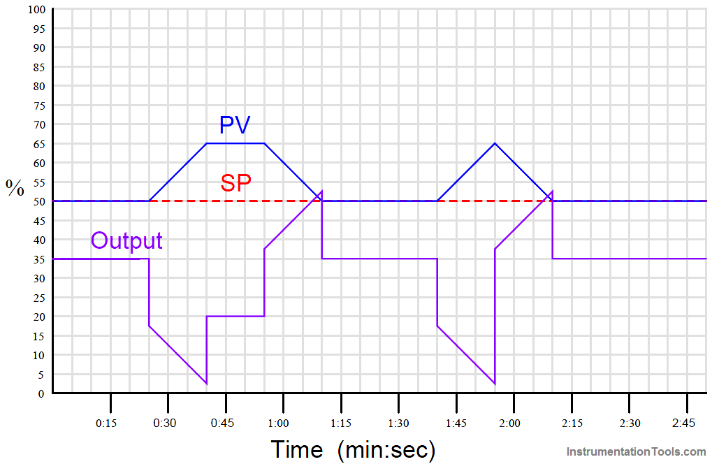
Suppose for example you were tasked with graphing the response of a PD (proportional + derivative) controller to the following PV and SP inputs over time.

You are told the controller has a gain of 1, a derivative time constant of 0.3 minutes, and is reverse-acting:

Proportional Derivative Controller Graph

My first recommendation is to qualitatively sketch the individual P and D responses. Simply draw two different trends, each one right above or below the given PV/SP trends, showing the shapes of each response over time.

You might even find it easier to do if you re-draw the original PV and SP trends on a piece of non-graph paper with the qualitative P and D trends also sketched on the same piece of non-graph paper.

The purpose of the qualitative sketches is to separate the task of determining shapes from the task of determining numerical values, in order to simplify the process.

After sketching the separate P and D trends, label each one of the “features” (changes either up or down) in these qualitative trends. This will allow you to more easily combine the effects into one output trend later:

PID Controller Graph

Now, you may qualitatively sketch an output trend combining each of these “features” into one graph.

Be sure to label each ramp or step originating with the separate P or D trends, so you know where each “feature” of the combined output graph originates from:

PD Controller Graph Analysis

Once the general shape of the output has been qualitatively determined, you may go back to the separate P and D trends to calculate numerical values for each of the labeled “features.”

Note that each of the PV ramps is 15% in height, over a time of 15 seconds (one-quarter of a minute). With a controller gain of 1, the proportional response to each of these ramps will also be a ramp that is 15% in height.

Taking our given derivative time constant of 0.3 minutes and multiplying that by the PV’s rate-of-change ( dPV/dt ) during each of its ramping periods (15% per one-quarter minute, or 60% per minute) yields a derivative response of 18% during each of the ramping periods. Thus, each derivative response “step” will be 18% in height.

Going back to the qualitative sketches of P and D actions, and to the combined (qualitative) output sketch, we may apply the calculated values of 15% for each proportional ramp and 18% for each derivative step to the labeled “features.”

We may also label the starting value of the output trend as given in the original problem (35%), to calculate actual output values at different points in time.

Calculating output values at specific points in the graph becomes as easy as cumulatively adding and subtracting the P and D “feature” values to the starting output value:

P+D Controller Graph

Now that we know the output values at all the critical points, we may quantitatively sketch the output trend on the original graph:

PID Controller Graph - 5

Credits : Tony R. Kuphaldt – Creative Commons Attribution 4.0 License

Don't Miss Our Updates
Be the first to get exclusive content straight to your email.
We promise not to spam you. You can unsubscribe at any time.
Invalid email address
You've successfully subscribed !

Continue Reading

Process Control Fundamentals
How to Analyze a Cascade Control Loop?
How to Configure a Smart Transmitter Using a HART Communicator?
Switch or Transmitter
Free PID Controller Gains Tuning Tool
Introduction to Modbus – Reading and Writing Data
Share This Article
Facebook Whatsapp Whatsapp LinkedIn Copy Link
Share
Leave a Comment

Leave a Reply Cancel reply

Your email address will not be published. Required fields are marked *

Stay Connected

128.3kFollowersLike
69.1kFollowersFollow
208kSubscribersSubscribe
38kFollowersFollow

Categories

Explore More

PLC or DCS Control System Spares
Instrument Loop Test Requirements and Operation Procedures
What is a Transducer ?
Instrumentation and Control (I&C) Design
Open Loop and Closed Loop Animation
DCS Controllers to Output Current Loops
PID Controller Response with different Input Signals
Ziegler-Nichols Open-Loop Method

Keep Learning

Internet of Things (IOT)

History of Internet of Things (IOT)

Process Dynamics and PID Controller Tuning

Process Dynamics and PID Controller Tuning

Sink or source PNP or NPN Normally Open or Normally Closed Input v. output. output

Sink or Source? Normally Open or Normally Closed?

Alarms to Annunciator

Basics of Alarms and Trips

feedforward control theory

Proportioning Feedforward action

Feedforward control with feedback trim

Feedforward Control Principle

PID Controller Loop Tuning Questions and Answers

PID Controller Loop Tuning Questions and Answers – Part 2

Feedforward with Dynamic Compensation - 3

Feedforward Control with Dynamic Compensation

Learn More

Siemens S7 300 CPU Status and LED Errors Explanation

Siemens S7 300 CPU Status and LED Errors Explanation

Ultrasonic Doppler Flow Meter Advantages and Disadvantages

Ultrasonic Doppler Flow Meter Advantages and Disadvantages

Magnetostrictive Level Transmitter Working Principle

Magnetostrictive Level Transmitter Working Principle

Valve Sequencing

Complementary Control Valve Sequence

Closed Loop Control System

Types of Control Systems

STAR DELTA Starter PLC Logic

STAR DELTA Programming using PLC Controller

Control Valves Pre-Commissioning Checklist

Control Valves Pre-Commissioning Checklist

Stripping tower unit

Process Control High Level Alarm Fault Analysis

Follow US
All rights reserved. Reproduction in whole or in part without written permission is prohibited.
Welcome Back!

Sign in to your account

Username or Email Address
Password

Lost your password?