Power Electronics – Phase Controlled Half Wave Rectifier RL Load

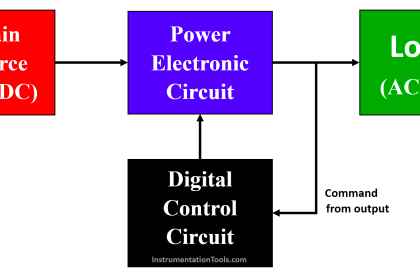
A phase-controlled half-wave rectifier with an RL load (resistor-inductor) is a circuit that converts AC voltage into a DC voltage.

In this circuit, a Thyristor is used to rectify the AC voltage, and an inductor (L) and a resistor (R) are connected in series to the Thyristor to form the RL load.

Phase Controlled Half Wave Rectifier RL

During the positive half-cycle of the input AC voltage, the thyristor is forward-biased and conducts when triggered. It allows current to flow through the RL load. At this point, the inductor stores energy.

During the negative half-cycle, the thyristor is reverse-biased and does not conduct. The diode (not shown in the diagram) conducts in reverse bias, allowing current to continue flowing through the load.

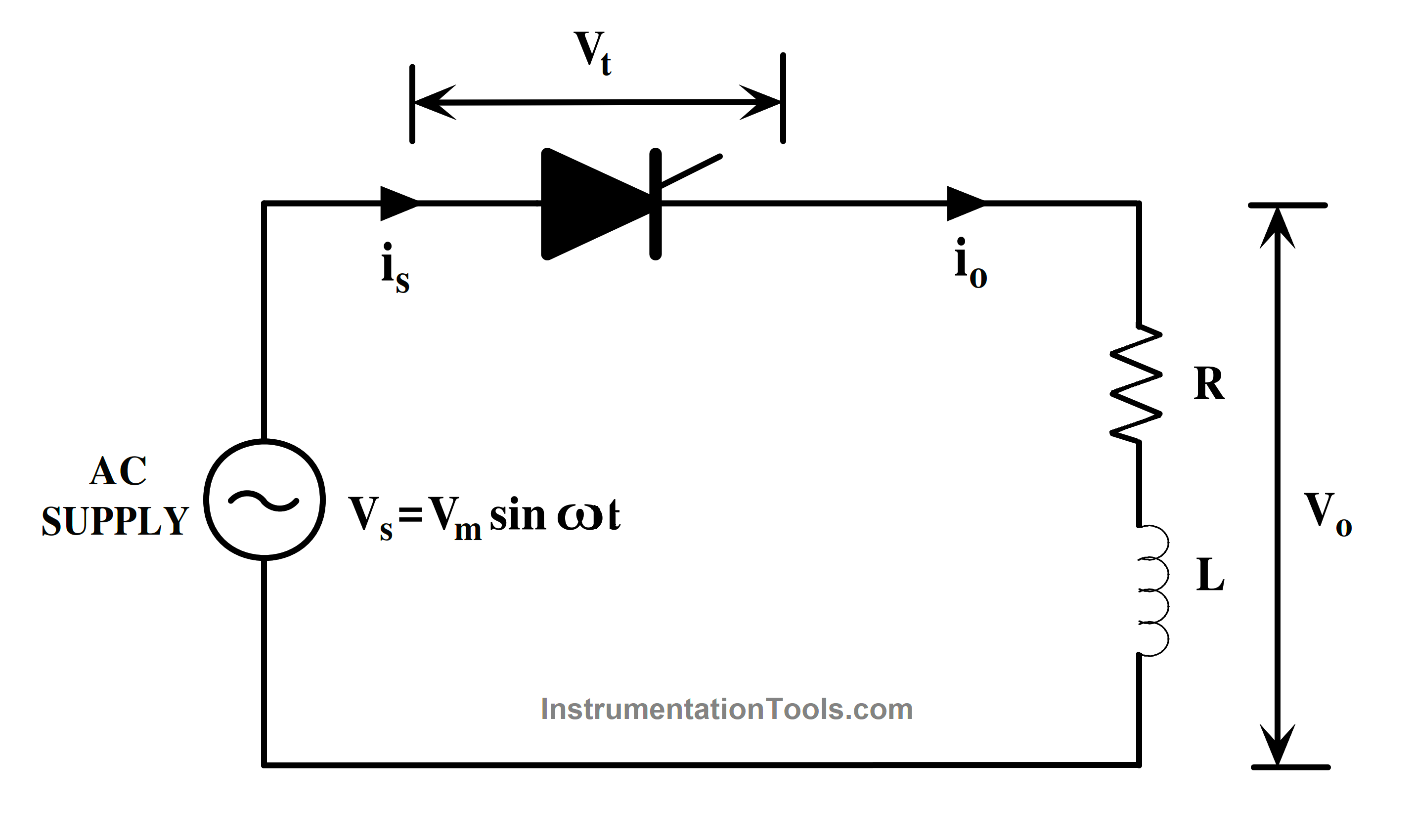
Fig. 1. Single Phase Half Controlled Rectifier

Circuit Components

The basic circuit diagram consists of the following components:

AC Power Supply: The input power source is typically an AC supply.

Thyristor (SCR): The thyristor acts as a controlled switch, allowing the current to flow in only one direction when it is triggered.

RL Load: The load is made up of an inductor (L) and a resistor (R) connected in series. The resistor represents the pure resistance of the load, and the inductor represents the inductive component.

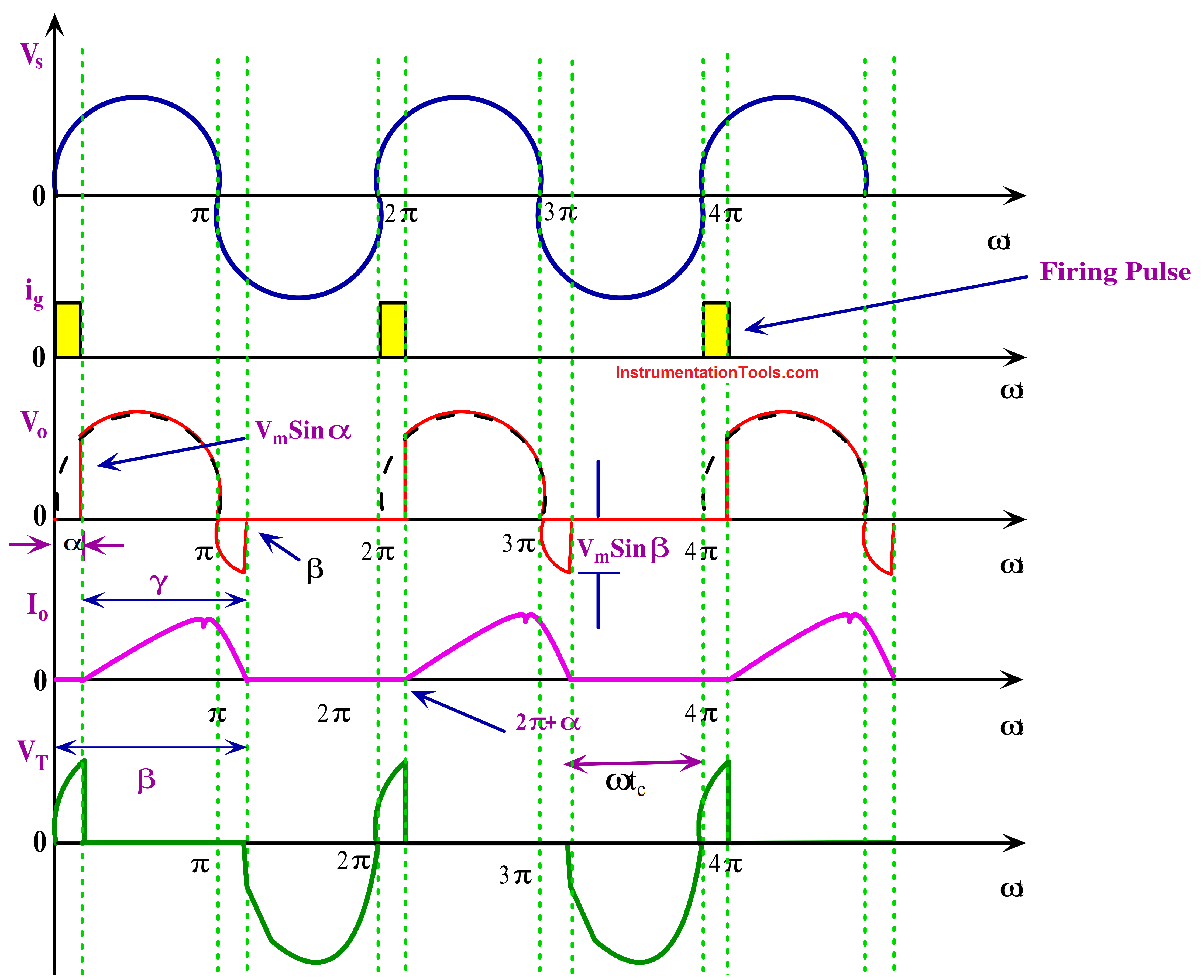
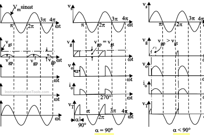
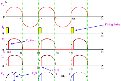
Fig. 2. Half-Controlled Rectifier Output With RL Load

Half-Controlled Rectifier Working

The thyristor T is supposed to be fired at an angle of ωt = α. When the thyristor T is activated at time ωt = α, an instantaneous load voltage equating to the source voltage develops across the load terminal. The thyristor is forward biased between ωt = 0 to α. Thus, as soon as the thyristor is gated, it begins to conduct.

But the current does not begin to flow at this point in the firing. This is just due to the load’s nature. The inductive nature of the load prevents any abrupt changes. As a result, the output current will be zero and increase gradually at time ωt = α. The output current will reach its maximum before beginning to decline. It should be emphasized that fully resistive loads do not exhibit this load current io behavior.

The load voltage Vo decreases to zero at time t. However, due to inductance L, the load current will not be zero at this precise moment. This causes the thyristor, despite being reverse-biased, to remain on. Instead, it will keep running until ωt = β. When the load current reaches zero at time ωt = β, the thyristor will turn off because it is reverse-biased. Natural commutation occurred in this situation.

Vo and io are equal to zero after ωt = β. At time ωt = (2π+α), the SCR is activated once more, vo is applied to the load, and the load current develops as previously elaborated. It is known as the extinction angle when the load current reaches zero, and it is known as the conduction angle when the thyristor is turned on.

The SCR is biased in the opposite direction from ωt = β to ωt = 2π. The current passing through the thyristor is zero at this time. Therefore, the circuit turn-off time is tc = [(2π – β) / ω] second. This period of time needs to be longer than the time required for the thyristor to turn off, or else the commutation will fail and the thyristor will switch on prematurely.

In Short

At wt=α

• The gate signal is used to activate the thyristor T. The source voltage vs and the load voltage V_o is instantly equal.
• However, the load or output current must gradually increase due to inductance L.
• I_o eventually achieves a maximum value and then starts to fall.

At wt= π

• Due to the load inductance L, V_o is zero but I_o is not.

After wt= π

• The SCR will not turn off even when the reverse anode voltage is applied after ωt= π because the load current io is greater than the holding current.
• Since Thyristor T is already reverse biased when I_o reduces to zero at some angle β>π, it turns off.

After wt=β

• V_o=0 and I_o =0 after ωt=β
• Angle β is referred to as the extinction angle, and angle γ= β-α is referred to as the conduction angle.

When ωt = α, V_T= Vm sinα from ωt = α to π, V_T = 0; and at ωt = π, V_T= Vm sin β, according to the waveform of voltage V_T across the thyristor T. VT is negative at ωt = β because β > π.

As a result, the thyristor has a reverse bias from ωt = β to 2π. Circuit turn-off time t_c, therefore, equals (2π- β)/α sec. The thyristor turn-off time, t_q, should be greater than t_c for satisfactory commutation.

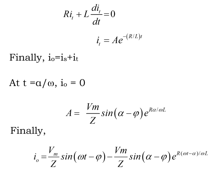
The circuit’s voltage equation is stated as

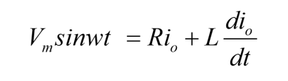
The load current i_o consists of two components, one i_s a steady-state component, and the other i_t is transient component i_t. Here is given by

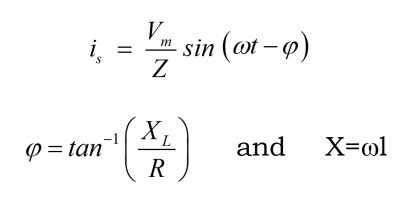
 Here, ϕ is the angle by which rms current Is lags Vs.

Transient component i_t can be obtained by simplifying the following equation

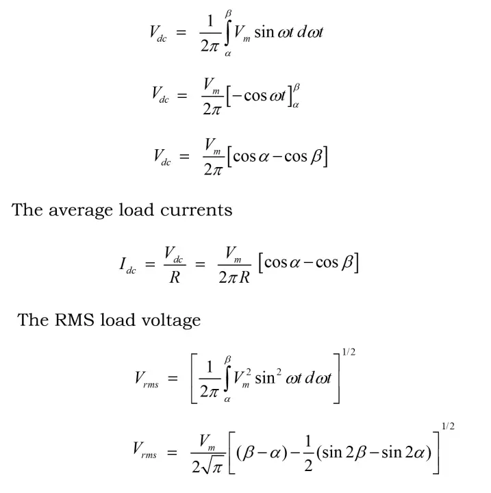
Analysis of Single-phase Half-controlled Rectifier With RL Load

The average load voltage Vo for the single-phase half-controlled rectifier is given by

Advantages of Phase Controlled Half Wave Rectifier

• Control over output voltage using the firing angle of the thyristor.
• Reduced harmonic distortion due to controlled switching.
• Smoothing effect due to the inductor, reducing ripple.
• Variable power delivery to the load

Disadvantages of Phase Controlled Half Wave Rectifier

• Voltage and current harmonics.
• Limited to resistive-inductive loads.
• Lower efficiency compared to fully controlled rectifiers due to the lagging power factor.
• More complex control circuitry compared to diode rectifiers

Matlab Source Code for Half-controlled Rectifier

% Parameters

R = 10; % Load resistance (in ohms)

L = 0.01; % Load inductance (in henries)

Vm = 100; % Peak voltage of the AC supply (in volts)

f = 50; % Frequency of the AC supply (in Hz)

w = 2*pi*f; % Angular frequency

% Simulation parameters

t = 0:0.0001:0.1; % Time vector (from 0 to 0.1 seconds with a step of 0.0001 seconds)

alpha = pi/3; % Firing angle (60 degrees in radians)

% Rectified output voltage calculation using a half-controlled rectifier formula

voltage = @(t, alpha) Vm * sqrt(2) * sin(w * t) - (sqrt(2) * Vm * sin(alpha) / (pi * (1 - cos(alpha)))) * cos(w * t - alpha);

% Current through RL load calculation

current = @(t, alpha) (sqrt(2) * Vm / (pi * R * (1 - cos(alpha)))) * (sin(w * t) - sin(alpha) * cos(w * t - alpha));

% Plot the input and output waveforms
% Plotting the waveforms
figure;

subplot(2,1,1);

plot(t, voltage(t, alpha), 'r');

title('Half-Controlled Rectifier Output Voltage');

xlabel('Time (s)');

ylabel('Voltage (V)');

grid on;

subplot(2,1,2);

plot(t, current(t, alpha), 'b');

title('Current through RL Load');

xlabel('Time (s)');

ylabel('Current (A)');

grid on;

Matlab Simulink Circuit

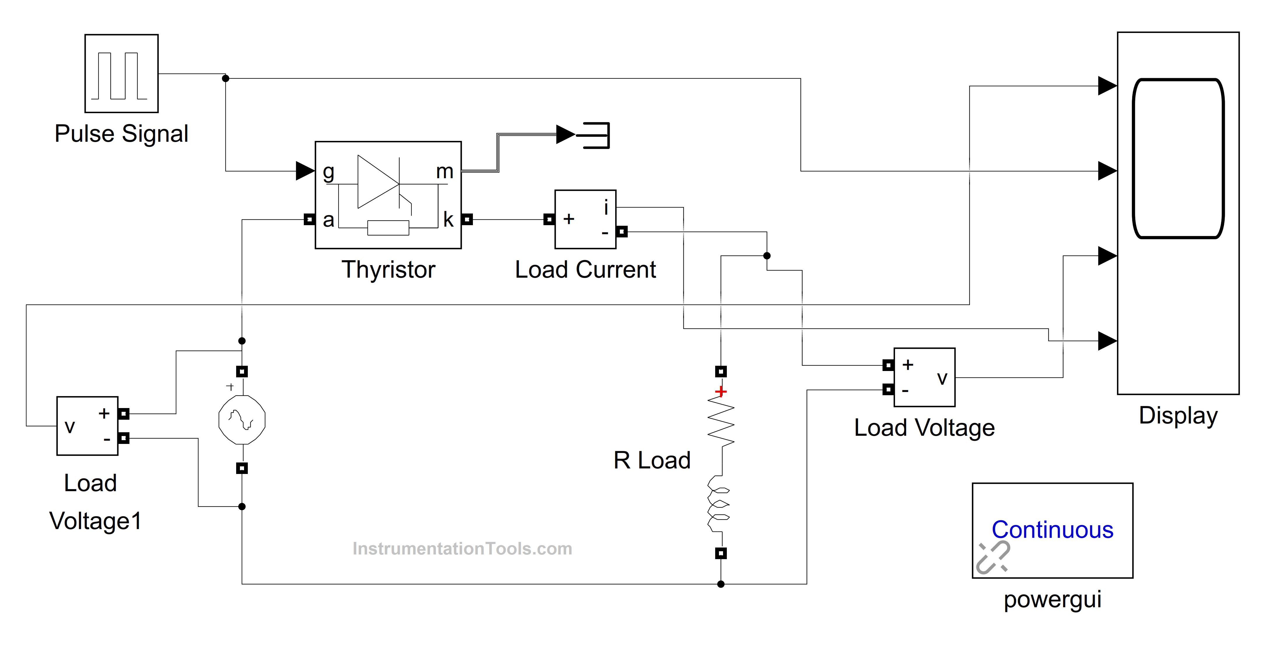
Fig.3. Simulink Circuit of Half-controlled Rectifier With RL Load

Simulink Result

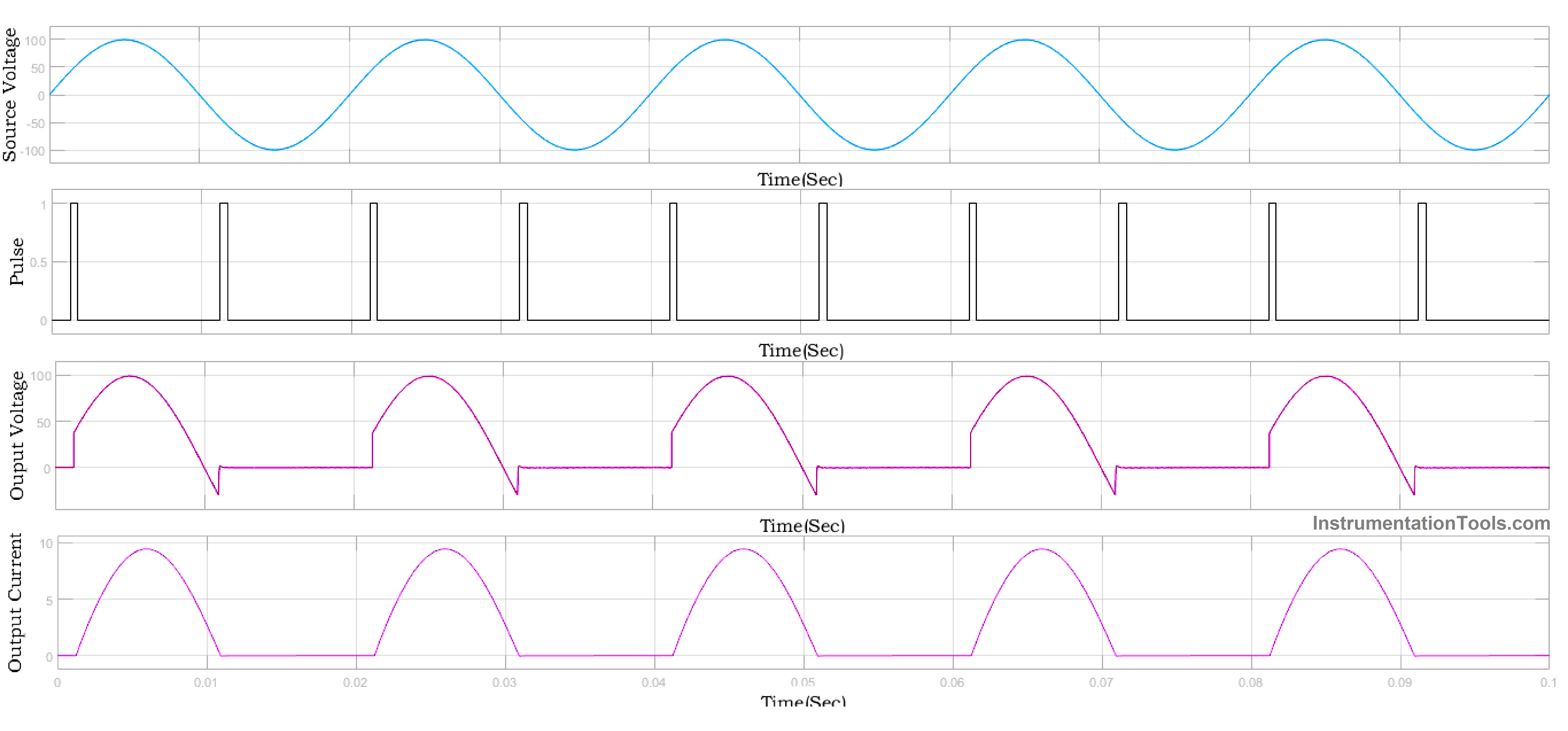
Fig.4. Simulink Response of Half-controlled Rectifier With RL Load

Reference

1. “Power Electronics” P. S. Bimbhra, Khanna Publishers, 2012
2. “Power Electronics: Circuits, Devices and Applications”, M H Rashid, Pearson     Education

If you liked this article, then please subscribe to our YouTube Channel for Instrumentation, Electrical, PLC, and SCADA video tutorials.

You can also follow us on Facebook and Twitter to receive daily updates.

Read Next:

• Thyristor Protection Circuits (SCR)
• Power Electronic Devices Specifications
• Half-Controlled Rectifier with R Load
• Top 100 Power Electronics Projects
• Thyristor Triggering Circuits and Types