When control valves operate between fully open and fully shut, they serve much the same purpose in process systems as resistors do in electric circuits: to dissipate energy. Like resistors, the form that this dissipated energy takes is mostly heat, although some of the dissipated energy manifests in the form of vibration and noise.
Valve noise may be severe in some cases, especially in certain gas flow applications. An important performance metric for control valves is noise production expressed in decibels (dB).
In most control valves, the dominant mechanism of energy dissipation comes as a result of turbulence introduced to the fluid as it travels through constrictive portions of the valve trim.
Basics of Control Valve Sizing
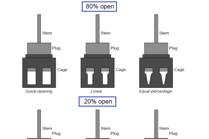
The following illustration shows these constrictive points within two different control valve types (shown by arrows):

The act of choosing an appropriate control valve for the expected energy dissipation is called valve sizing.
Physics of energy dissipation in a turbulent fluid stream
Control valves are rated in their ability to throttle fluid flow much in the same way resistors are rated in their ability to throttle the flow of electrons in a circuit.
For resistors, the unit of measurement for electron flow restriction is the ohm: 1 ohm of resistance results in a voltage drop of 1 volt across that resistance given a current through the resistance equal to 1 ampere:


Where,
R = Electrical resistance in ohms
V = Electrical voltage drop in volts
I = Electrical current in amperes
Ohm’s Law is a simple, linear relationship, expressing the “friction” encountered by electric charge carriers as they slowly drift through a solid object.
When a fluid moves turbulently through any restriction, energy is inevitably dissipated in that turbulence.
The amount of energy dissipated is proportional to the kinetic energy of the turbulent motion, which is proportional to the square of velocity according to the classic kinetic energy equation for moving objects:

If we were to re-write this equation to express the amount of kinetic energy represented by a volume of moving fluid with velocity v, it would look like this:

We know that the amount of energy dissipated by turbulence in such a fluid stream will be some proportion (k) of the total kinetic energy, so:
 Any energy lost in turbulence eventually manifests as a loss in fluid pressure downstream of that turbulence.
Thus, a control valve throttling a fluid flowstream will have a greater upstream pressure than downstream pressure (assuming all other factors such as pipe size and height above ground level being the same downstream as upstream):

This pressure drop (P1 − P2, or ΔP) is equivalent to the voltage drop seen across any current carrying resistor, and may be substituted for dissipated energy per unit volume in the previous equation.
We may also substitute Q/A for velocity v because we know volumetric flow rate (Q) is the product of fluid velocity and pipe cross-section area (Q = Av) for incompressible fluids such as liquids:

Next, we will solve for a quotient with pressure drop (P1 − P2) in the numerator and flow rate (Q) in the denominator so the equation bears a resemblance to Ohm’s Law (R = V/I ):

Either side of the last equation represents a sort of “Ohm’s Law” for turbulent liquid restrictions: the left-hand side expressing fluid “resistance” in the state variables of pressure drop and volumetric flow, and the right-hand term expressing fluid “resistance” as a function of fluid density and restriction geometry.
We can see how pressure drop (P1 − P2) and volumetric flow rate (Q) are not linearly related as voltage and current are for resistors, but that nevertheless we still have a quantity that acts like a “resistance” term:

Where,
R = Fluid “resistance”
P1 = Upstream fluid pressure
P2 = Downstream fluid pressure
Q = Volumetric fluid flow rate
k = Turbulent energy dissipation factor
ρ = Mass density of fluid
A = Cross-sectional area of restriction
The fluid “resistance” of a restriction depends on several variables: the proportion of kinetic energy lost due to turbulence (k), the density of the fluid (ρ), and the cross-sectional area of the restriction (A).
In a control valve throttling a liquid flow stream, only the first and last variables are subject to change with stem position, fluid density remaining relatively constant.
In a wide-open control valve, especially valves offering a nearly unrestricted path for moving fluid (e.g. ball valves, eccentric disk valves), the value of A will be at a maximum value essentially equal to the pipe’s area, and k will be nearly zero. In a fully shut control valve, A is zero, creating a condition of infinite “resistance” to fluid flow.
It is customary in control valve engineering to express the “restrictiveness” of any valve in terms of how much flow it will pass given a certain pressure drop and fluid specific gravity (Gf ).
This measure of valve performance is called flow capacity or flow coefficient, symbolized as Cv. A greater flow capacity value represents a less restrictive (less “resistive”) valve, able to pass greater rates of flow for the same pressure drop.
This is analogous to expressing an electrical resistor’s rating in terms of conductance (G) rather than resistance (R): how many amperes of current it will pass with 1 volt of potential drop (I = GV instead of I = V/R).
If we return to one of our earlier equations expressing pressure drop in terms of flow rate, restriction area, dissipation factor, and density, we will be able to manipulate it into a form expressing flow rate (Q) in terms of pressure drop and density, collecting k and A into a third term which will become flow capacity (Cv):
First, we must substitute specific gravity (Gf ) for mass density (ρ) using the following definition of specific gravity:
 Control Valve Sizing Equation")
The first square-rooted term in the equation, √(2A2/kpwater) , is the valve capacity or Cv factor. Substituting Cv for this term results in the simplest form of valve sizing equation (for incompressible fluids):

Where,
Q = Volumetric flow rate of liquid (gallons per minute, GPM)
Cv = Flow coefficient of valve
P1 = Upstream pressure of liquid (PSI)
P2 = Downstream pressure of liquid (PSI)
Gf = Specific gravity of liquid (ratio of liquid density to standard water density)
In the United States of America, Cv is defined as the number of gallons per minute of water that will flow through a valve with 1 PSI of pressure drop.
A similar valve capacity expression used with metric units rates valves in terms of how many cubic meters per hour of water will flow through a valve with a pressure drop of 1 bar. This latter flow capacity is symbolized as Kv.
For the best results predicting required Cv values for control valves in any service, it is recommended that you use valve sizing software provided by control valve manufacturers.
The formulae shown here do not account for all factors (Such factors include fluid compressibility, viscosity, specific heat, vapor pressure etc) influencing fluid flow rate and pressure drop, and therefore yield approximate values only.
Modern valve sizing software is easy to use, especially when referenced to specific models of control valve sold by that manufacturer, and is able to account for a diverse multitude of factors affecting proper sizing.


thanks very much