Magnetic Circuits
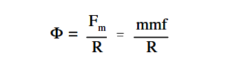
A magnetic circuit can be compared with an electric current in which EMF, or voltage, produces a current flow. The ampere-turns (NI), or the magnetomotive force (Fm or mmf), will produce a magnetic flux Φ (Figure 26). The mmf can be compared with EMF, and the flux (Φ) can be compared to current.
The below Equation is the mathematical representation of magnetomotive force derived using Ohm’s Law,
I = E / R
where
Φ = magnetic flux, Wb
Fm = magnetomotive force (mmf), At
R = reluctance, At/Wb
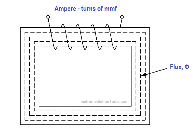
Figure 26 – Magnetic Current with Closed Iron Path
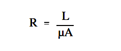
The below Equation is the mathematical representation for reluctance.
where
R = reluctance, At/Wb
L = length of coil, m
µ = permeability of magnetic material, ( (T – m) / At)
A = cross-sectional area of coil, m2
Example: A coil has an mmf of 600 At, and a reluctance of 3×10⁶ At/Wb. Find the total flux Φ
Solution:
Φ = mmf / R =
Φ = 600 At / (3×10⁶ )At/Wb = 200 µ Wb
BH Magnetization Curve
The BH Magnetization Curve (Figure 27) shows how much flux density (B) results from increasing the flux intensity (H). The curves in Figure 27 are for two types of soft iron cores plotted for typical values. The curve for soft iron 1 shows that flux density B increases rapidly with an increase in flux intensity H, before the core saturates, or develops a “knee.” Thereafter, an increase in flux intensity H has little or no effect on flux density B. Soft iron 2 needs a much larger increase in flux intensity H before it reaches its saturation level at H = 5000 At/m, B = 0.3 T.
Air, which is nonmagnetic, has a very low BH profile, as shown in Figure 27.
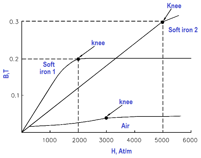
Figure 27 Typical BH Curve for Two Types of Soft Iron
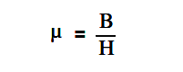
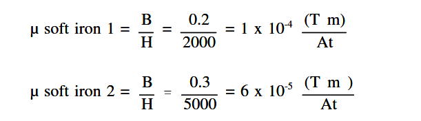
The permeability (µ) of a magnetic material is the ratio of B to H.
The below Equation is the mathematical representation for magnetic material permeability.
The average value of permeability is measured where the saturation point, or knee, is first established. Figure 27 shows that the normal or average permeability for the two irons as follows.
In SI units, the permeability of a vacuum is µo =4πx10-7 H/m or 1.26 x 10⁻⁶ or T-m/At. In order to calculate permeability, the value of relative permeability µr must be multiplied by µo .
Equation is the mathematical representation for permeability.
µ = µr x µo
Example: Find the permeability of a material that has a relative permeability of 100.
µ = µr x µo
= 100 ( 1.26 x 10⁻⁶ ) T-m/At
Hysteresis
When current in a coil reverses direction thousands of times per second, hysteresis can cause considerable loss of energy. Hysteresis is defined as “a lagging behind.” The magnetic flux in an iron core lags behind the magnetizing force.
The hysteresis loop is a series of curves that shows the characteristics of a magnetic material (Figure 28). Opposite directions of current will result in opposite directions of flux intensity shown as +H and -H. Opposite polarities are also shown for flux density as +B or -B. Current starts at the center (zero) when unmagnetized.
Positive H values increase B to the saturation point, or +Bmax , as shown by the dashed line. Then H decreases to max zero, but B drops to the value of Br due to hysteresis. By reversing the original current, H now becomes negative. B drops to zero and continues on to -Bmax.
As the -H values decrease (less negative), B is reduced to -B max when H is zero. With a positive swing of current, H once again becomes positive, producing saturation at +Bmax. The hysteresis loop is completed. The loop does not return to zero because of hysteresis.
The value of +Br or -Br , which is the flux density remaining after the magnetizing force is zero, is called the retentivity of that magnetic material. The value of -Hc , which is the force that must be applied in the reverse direction to reduce flux density to zero, is called the coercive force of the material.
The greater the area inside the hysteresis loop, the larger the hysteresis losses.
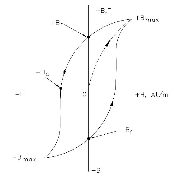
Figure 28 – Hysteresis Loop for Magnetic Materials
Magnetic Induction
Electromagnetic induction was discovered by Michael Faraday in 1831. Faraday found that if a conductor “cuts across” lines of magnetic force, or if magnetic lines of force cut across a conductor, a voltage, or EMF, is induced into the conductor. Consider a magnet with its lines of force from the North Pole to the South Pole (Figure 29). A conductor C, which can be moved between the poles of the magnet, is connected to a galvanometer G, which can detect the presence of voltage, or EMF. When the conductor is not moving, zero EMF is indicated by the galvanometer.
If the conductor is moving outside the magnetic field at position 1, zero EMF is still indicated by the galvanometer. When the conductor is moved to position 2, the lines of magnetic force will be cut by the conductor, and the galvanometer will deflect to point A. Moving the conductor to position 3 will cause the galvanometer to return to zero. By reversing the direction in which the conductor is moved (3 to 1), the same results are noticed, but of opposite polarity. If we hold the conductor stationary in the magnetic lines of force, at position 2, the galvanometer indicates zero. This fact shows that there must be relative motion between the conductor and the magnetic lines of force in order to induce an EMF.
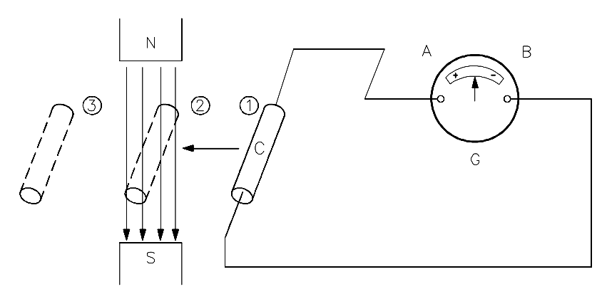
Figure 29 – Induced EMF
The most important application of relative motion is seen in electric generators. In a DC generator, electromagnets are arranged in a cylindrical housing. Conductors, in the form of coils, are rotated on a core such that the coils continually cut the magnetic lines of force. The result is a voltage induced in each of the conductors. These conductors are connected in series, and the induced voltages are added together to produce the generator’s output voltage.
Faraday’s Law of Induced Voltage
The magnitude of the induced voltage depends on two factors:
- the number of turns of a coil, and
- how fast the conductor cuts across the magnetic lines of force, or flux.
The below Equation is the mathematical representation for Faraday’s Law of Induced Voltage.
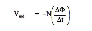
where
Vind = induced voltage, V
N = number of turns in a coil
∆Φ/∆t= rate at which the flux cuts across the conductor, Wb/s
Example 1:
Given: Flux = 4 Wb. The flux increases uniformly to 8 Wb in a period of 2 seconds. Find induced voltage in a coil that has 12 turns, if the coil is stationary in the magnetic field.
Solution:
∆Φ = 8Wb – 4Wb = 4Wb
∆t= 2s
then ∆Φ/∆t = 4Wb / 2s = 2Wb/ s
Vind = -12 (2) = -24 volts
Example 2: In Example 1, what is the induced voltage, if the flux remains 4 Wb after 2 s?
Solution:
V ind = – 12 (0/2) = 0 volts
No voltage is induced in Example 2. This confirms the principle that relative motion must exist between the conductor and the flux in order to induce a voltage.
Lenz’s Law
Lenz’s Law determines the polarity of the induced voltage. Induced voltage has a polarity that will oppose the change causing the induction. When current flows due to the induced voltage, a magnetic field is set up around that conductor so that the conductor’s magnetic field reacts with the external magnetic field.
This produces the induced voltage to oppose the change in the external magnetic field. The negative sign in above equation is an indication that the emf is in such a direction as to produce a current whose flux, if added to the original flux, would reduce the magnitude of the emf.