If a square-wave signal is applied to an RC passive integrator circuit, the output signal will appear to have a “sawtooth” shape, the crisp rising and falling edges of the square wave replaced by damped curves:
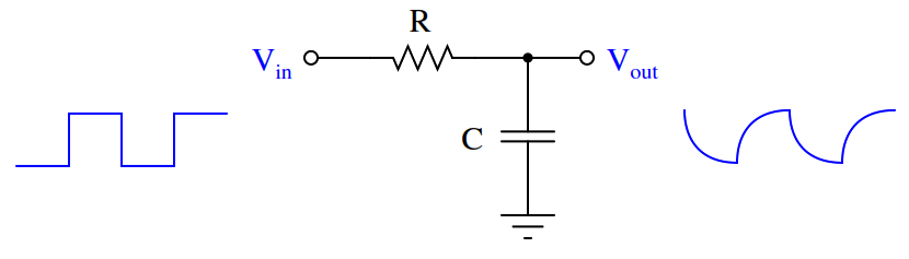
In a word, the output signal of this circuit lags behind the input signal, unable to keep pace with the steep rising and falling edges of the square wave.
Most mechanical and chemical processes exhibit a similar tendency: an “inertial” opposition to rapid changes. Even instruments themselves naturally (Note) damp sudden stimuli. We could have just as easily subjected a pressure transmitter to a series of pressure pulses resembling square waves, and witnessed the output signal exhibit the same damped response:
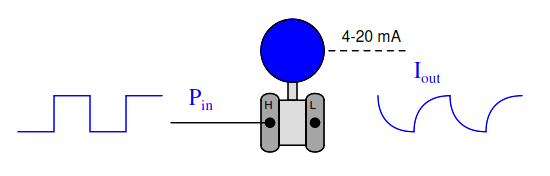
Note : It is also possible to configure many instruments to deliberately damp their response to input conditions. This is called damping.
The gravity-drained level-control process highlighted in an earlier subsection exhibits a very similar response to a sudden change in control valve position:
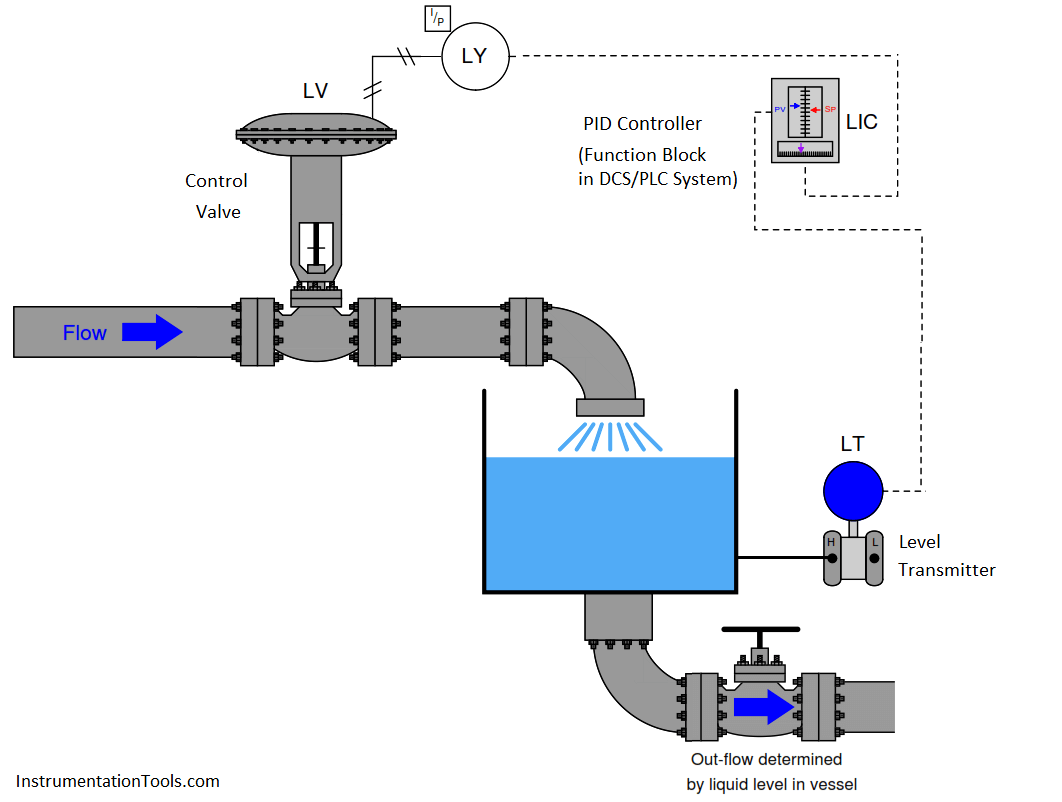
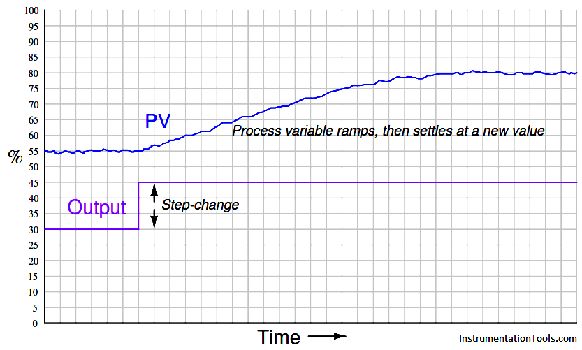
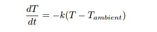
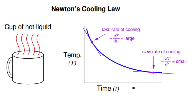
For any particular flow rate into the vessel, there will be a final (self-regulating) point where the liquid level “wants” to settle (Note) . However, the liquid level does not immediately achieve that new level if the control valve jumps to some new position, owing to the “capacity” of the vessel and the dynamics of gravity flow. Any physical behavior exhibiting the same “settling” behavior over time may be said to illustrate a first-order lag. A classic “textbook” example of a first-order lag is the temperature of a cup of hot liquid, gradually equalizing with room temperature. The liquid’s temperature drops rapidly at first, but then slows its approach to ambient temperature as time progresses. This natural tendency is described by Newton’s Law of Cooling, mathematically represented in the form of a differential equation (an equation containing a variable along with one or more of its derivatives). In this case, the equation is a first-order differential equation, because it contains the variable for temperature (T) and the first derivative of temperature ( dT/dt ) with respect to time:
Note : 11 Assuming a constant discharge valve position. If someone alters the hand valve’s position, the relationship between incoming flow rate and final liquid level changes.
Where,
T = Temperature of liquid in cup
Tambient = Temperature of the surrounding environment
k = Constant representing the thermal conductivity of the cup
t = Time
All this equation tells us is that the rate of cooling ( dT/dt ) is directly proportional (−k) to the difference in temperature between the liquid and the surrounding air (T −Tambient ). The hotter the temperature, the faster the object cools (the faster rate of temperature fall):
The proportionality constant in this equation (k) represents how readily thermal energy escapes the hot cup. A cup with more thermal insulation, for example, would exhibit a smaller k value (i.e. the rate of temperature loss dT/dt will be less for any given temperature difference between the cup and ambient T − T ambient ).
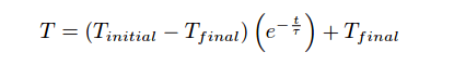
A general solution to this equation is as follows:
Where,
T = Temperature of liquid in cup at time t
Tinitial = Starting temperature of liquid (t = 0)
Tfinal = Ultimate temperature of liquid (ambient)
e = Euler’s constant
τ = “Time constant” of the system
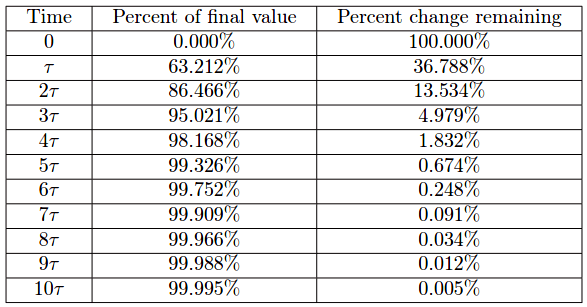
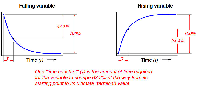
This mathematical analysis introduces a descriptive quantity of the system: something called a time constant. The “time constant” of a first-order system is the amount of time necessary for the system to come to within 36.8% (e−1 ) of its final value (i.e. the time required for the system to go 63.2% of the way from the starting point to its ultimate settling point: 1 − e−1 ). After two time-constants’ worth of time, the system will have come to within 13.5% (e−2 ) of its final value (i.e. gone 86.5% of the way: 1 −e−2 ); after three time-constants’ worth of time, to within 5% (e ) of the final value, (i.e. gone 95% of the way: 1 − e−3 ). After five time-constants’ worth of time, the system will be within 1% (e−5 , rounded to the nearest whole percent) of its final value, which is often close enough to consider it “settled” for most practical purposes.
The concept of a “time constant” may be shown in graphical form for both falling and rising variables:
Students of electronics will immediately recognize this concept, since it is widely used in the analysis and application of capacitive and inductive circuits. However, you should recognize the fact that the concept of a “time constant” for capacitive and inductive electrical circuits is only one case of a more general phenomenon. Literally any physical system described by the same first-order differential equation may be said to have a “time constant.” Thus, it is perfectly valid for us to speak of a hot cup of coffee as having a time constant (τ ), and to say that the coffee’s temperature will be within 1% of room temperature after five of those time constants have elapsed.
In the world of process control, it is more customary to refer to this as a lag time than as a time constant, but these are really interchangeable terms. The term “lag time” makes sense if we consider a first-order system driven to achieve a constant rate of change. For instance, if we subjected our RC circuit to a ramping input voltage rather than a “stepped” input voltage – such that the output ramped as well instead of passively settling at some final value – we would find that the amount of time separating equal input and output voltage values was equal to this time constant (in an RC circuit, τ = RC):
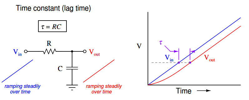
Lag time is thus defined as the difference in time between when the process variable ramps to a certain value and when it would have ramped to that same value were it not for the existence of first-order lag in the system. The system’s output variable lags behind the ramping input variable by a fixed amount of time, regardless of the ramping rate. If the process in question is an RC circuit, the lag time will still be the product of (τ = RC), just as the “time product” defined for a stepped input voltage. Thus, we see that “time constant” and “lag time” are really the exact same concept, merely manifesting in different forms as the result of two different input conditions (stepped versus ramped).
When an engineer or a technician describes a process being “fast” or “slow,” they generally refer to the magnitude of this lag time. This makes lag time very important to our selection of PID controller tuning values. Integral and derivative control actions in particular are sensitive to the amount of lag time in a process, since both those actions are time-based. “Slow” processes (i.e. process types having large lag times) cannot tolerate aggressive integral action, where the controller “impatiently” winds the output up or down at a rate that is too rapid for the process to respond to. Derivative action, however, is generally useful on processes having large lag times.