Instrument Zero and Span Calibration

Every instrument has at least one input and one output. For a pressure sensor, the input would be some fluid pressure and the output would (most likely) be an electronic signal. For a loop indicator, the input would be a 4-20 mA current signal and the output would be a human-readable display. For a variable-speed motor drive, the input would be an electronic signal and the output would be electric power to the motor.

Calibration and ranging are two tasks associated with establishing an accurate correspondence between any instrument’s input signal and its output signal.

Simply defined, calibration assures the instrument accurately senses the real-world variable it is supposed to measure or control. Simply defined, ranging establishes the desired relationship between an instrument’s input and its output.

Calibration versus Re-ranging

To calibrate an instrument means to check and adjust (if necessary) its response so the output accurately corresponds to its input throughout a specified range. In order to do this, one must expose the instrument to an actual input stimulus of precisely known quantity.

For a pressure gauge, indicator, or transmitter, this would mean subjecting the pressure instrument to known fluid pressures and comparing the instrument response against those known pressure quantities. One cannot perform a true calibration without comparing an instrument’s response to known, physical stimuli.

To range an instrument means to set the lower and upper range values so it responds with the desired sensitivity to changes in input. For example, a pressure transmitter set to a range of 0 to 200 PSI (0 PSI = 4 mA output ; 200 PSI = 20 mA output) could be re-ranged to respond on a scale of 0 to 150 PSI (0 PSI = 4 mA ; 150 PSI = 20 mA).

In analog instruments, re-ranging could (usually) only be accomplished by re-calibration, since the same adjustments were used to achieve both purposes.

In digital instruments, calibration and ranging are typically separate adjustments (i.e. it is possible to re-range a digital transmitter without having to perform a complete recalibration), so it is important to understand the difference.

Zero and span adjustments

The purpose of calibration is to ensure the input and output of an instrument reliably correspond to one another throughout the entire range of operation. We may express this expectation in the form of a graph, showing how the input and output of an instrument should relate.

For the vast majority of industrial instruments this graph will be linear:

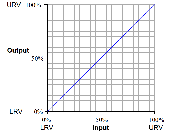
This graph shows how any given percentage of input should correspond to the same percentage of output, all the way from 0% to 100%.

Things become more complicated when the input and output axes are represented by units of measurement other than “percent.” Take for instance a pressure transmitter, a device designed to sense a fluid pressure and output an electronic signal corresponding to that pressure.

Here is a graph for a pressure transmitter with an input range of 0 to 100 pounds per square inch (PSI) and an electronic output signal range of 4 to 20 milliamps (mA) electric current:

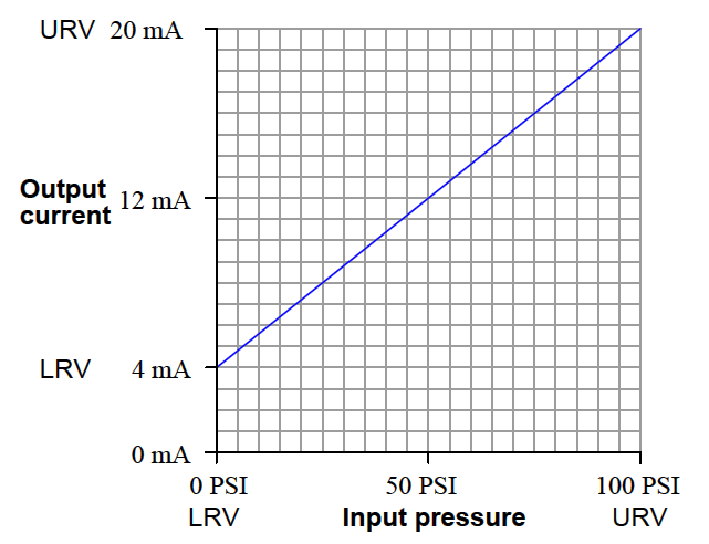
Although the graph is still linear, zero pressure does not equate to zero current. This is called a live zero, because the 0% point of measurement (0 PSI fluid pressure) corresponds to a non-zero (“live”) electronic signal. 0 PSI pressure may be the LRV (Lower Range Value) of the transmitter’s input, but the LRV of the transmitter’s output is 4 mA, not 0 mA.

Any linear, mathematical function may be expressed in “slope-intercept” equation form:

y = mx + b

Where,
y = Vertical position on graph
x = Horizontal position on graph
m = Slope of line
b = Point of intersection between the line and the vertical (y) axis

This instrument’s calibration is no different. If we let x represent the input pressure in units of PSI and y represent the output current in units of milliamps, we may write an equation for this instrument as follows:

y = 0.16x + 4

On the actual instrument (the pressure transmitter), there are two adjustments which let us match the instrument’s behavior to the ideal equation. One adjustment is called the zero while the other is called the span.

These two adjustments correspond exactly to the b and m terms of the linear function, respectively: the “zero” adjustment shifts the instrument’s function vertically on the graph (b), while the “span” adjustment changes the slope of the function on the graph (m). By adjusting both zero and span, we may set the instrument for any range of measurement within the manufacturer’s limits.

The relation of the slope-intercept line equation to an instrument’s zero and span adjustments reveals something about how those adjustments are actually achieved in any instrument.

A “zero” adjustment is always achieved by adding or subtracting some quantity, just like the y-intercept term b adds or subtracts to the product mx. A “span” adjustment is always achieved by multiplying or dividing some quantity, just like the slope m forms a product with our input variable x.

Zero adjustments typically take one or more of the following forms in an instrument:

• Bias force (spring or mass force applied to a mechanism)
• Mechanical offset (adding or subtracting a certain amount of motion)
• Bias voltage (adding or subtracting a certain amount of potential)

Span adjustments typically take one of these forms:

• Fulcrum position for a lever (changing the force or motion multiplication)
• Amplifier gain (multiplying or dividing a voltage signal)
• Spring rate (changing the force per unit distance of stretch)

It should be noted that for most analog instruments, zero and span adjustments are interactive. That is, adjusting one has an effect on the other.

Specifically, changes made to the span adjustment almost always alter the instrument’s zero point1. An instrument with interactive zero and span adjustments requires much more effort to accurately calibrate, as one must switch back and forth between the lower- and upper-range points repeatedly to adjust for accuracy.