While the term “probability” may evoke images of imprecision, probability is in fact an exact mathematical concept: the ratio a specific outcome to total possible outcomes where 1 (100%) represents certainty and 0 (0%) represents impossibility.
A probability value between 1 and 0 describes an outcome that occurs some of the time but not all of the time.
Reliability – which is the expression of how likely a device or a system is to function as intended – is based on the mathematics of probability. Therefore, a rudimentary understanding of probability mathematics is necessary to grasp what reliability means.
Before we dig too deeply into discussions of reliability, some definition of terms is in order. We have defined “reliability” to mean the probability of a device or system functioning as designed, which is a good general definition but sometimes not specific enough for our needs.
There are usually a variety of different ways in which a device or system can fail, and these different failure modes usually have different probability values. Let’s take for example a fire alarm system triggered by a manual pushbutton switch: the intended function of such a system is to activate an alarm whenever the switch is pressed.
If we wish to express the reliability of this system, we must first carefully define what we mean by “failure”. One way in which this simple fire alarm system could fail is if it remained silent when the pushbutton switch was pressed (i.e. not alerting people when it should have).
Another, completely different, way this simple system could fail is by accidently sounding the alarm when no one pressed the switch (i.e. alerting people when it had no reason to, otherwise known as a “false alarm”). If we discuss the “reliability” of this fire alarm system, we may need to differentiate between these two different kinds of unreliable system behaviors.
The electrical power industry has an interest in ensuring the safe delivery of electrical power to loads, both ensuring maximum service to customers while simultaneously shutting power off as quickly as possible in the event of dangerous system faults.
A complex system of fuses, circuit breakers, and protective relays work together to ensure the flow of power remains uninterrupted as long as safely possible. These protective devices must shut off power when they sense dangerous conditions, but they must also refrain from needlessly shutting off power when there is no danger.
Like our fire alarm system which must alert people when needed yet not sound false alarms, electrical protective systems serve two different needs. In order to avoid confusion when quantifying the reliability of electrical protective systems to function as designed, the power industry consistently uses the following terms:
- Dependability: The probability a protective system will shut off power when needed
- Security: The probability a protective system will allow power to flow when there is no danger
- Reliability: A combination of dependability and security
For the sake of clarity I will use these same terms when discussing the reliability of any instrument or control systems. “Dependability” is how reliably a device or system will take appropriate action when it is actively called to do so – in other words, the degree to which we may depend on this device or system to do its job when activated.
“Security” is how reliably a device or system refrains from taking action when no action should be taken – in other words, the degree to which we may feel secure it won’t needlessly trigger a system shutdown or generate a false alarm. If there is no need to differentiate, the term “reliability” will be used as a general description of how probable a device or system will do what it was designed to do.
Safety Instrumented System Probability
The following matrix should help clarify the meanings of these three terms, defined in terms of what the protective component or system does under various conditions:

In summary: a protective function that does not trip when it doesn’t need to is secure; a protective function that trips when it needs to is dependable; a protective system that does both is reliable.
The Boolean variables used to symbolize dependability (D), security (S), undependability (D), and unsecurity (S) tell us something about the relationships between those four quantities. A bar appearing over a Boolean variable represents the complement of that variable.
For example, security (S) and unsecurity (S) are complementary to each other: if we happen to know the probability that a device or system will be secure, then we may calculate with assurance the probability that it is unsecure.
A fire alarm system that is 99.3% secure (i.e. 99.3% of the time it generates no false alarms) must generate false alarms the other 0.7% of the time in order to account for all possible system responses 100% of the time no fires occur.
If that same fire alarm system is 99.8% dependable (i.e. it alerts people to the presence of a real fire 99.8% of the time), then we may conclude it will fail to report 0.02% of real fire incidents in order to account for all possible responses during 100% of fire incidents.
However, it should be clearly understood that there is no such simple relationship between security (S) and dependability (D) because these two measures refer to completely different conditions and (potentially) different modes of failure.
The specific faults causing a fire alarm system to generate a false alarm (an example of an unsecure outcome, S) are quite different from the faults disabling that same fire alarm system in the event of a real fire (an example of an undependable outcome, D).
Through the application of redundant components and clever system design we may augment dependability and/or security (sometimes improving one at the expense of the other), but it should be understood that these are really two fundamentally different probability measures and as such are not necessarily related.
Mathematical Probability
Probability may be defined as a ratio of specific outcomes to total (possible) outcomes. If you were to flip a coin, there are really only two possibilities (coin could also land on its edge, which is a third possibility.
However, that third possibility is so remote as to be negligible) for how that coin may land: face-up (“heads”) or face-down (“tails”). The probability of a coin falling “tails” is thus one-half ( 1/2 ),
since “tails” is one specific outcome out of two total possibilities. Calculating the probability (P) is a matter of setting up a ratio of outcomes:
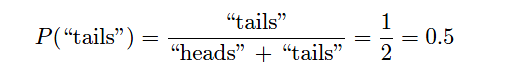
This may be shown graphically by displaying all possible outcomes for the coin’s landing (“heads” or “tails”), with the one specific outcome we’re interested in (“tails”) highlighted for emphasis:

The probability of the coin landing “heads” is of course exactly the same, because “heads” is also one specific outcome out of two total possibilities.
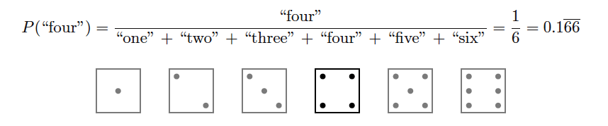
If we were to roll a six-sided die, the probability of that die landing on any particular side (let’s arbitrarily choose the “four” side) is one out of six, because we’re looking at one specific outcome out of six total possibilities:
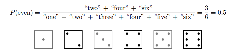
If we were to roll the same six-sided die, the probability of that die landing on an even-numbered side (2, 4, or 6) is three out of six, because we’re looking at three specific outcomes out of six total possibilities:
As a ratio of specific outcomes to total possible outcomes, the probability of any event will always be a number ranging in value from 0 to 1, inclusive.
This value may be expressed as a fraction ( 1/2 ), as a per unit value (0.5), as a percentage (50%), or as a verbal statement (e.g. “three out of six”).
A probability value of zero (0) means a specific event is impossible, while a probability of one (1) means a specific event is guaranteed to occur.
Probability values realistically apply only to large samples. A coin tossed ten times may very well fail to land “heads” exactly five times and land “tails” exactly five times. For that matter, it may fail to land on each side exactly 500000 times out of a million tosses.
However, so long as the coin and the coin-tossing method are fair (i.e. not biased in any way), the experimental results will approach the ideal probability value as the number of trials approaches infinity. Ideal probability values become less and less certain as the number of trials decreases, and are completely useless for singular (non-repeating) events.
A familiar application of probability values is the forecasting of meteorological events such as rainfall. When a weather forecast service provides a rainfall prediction of 65% for a particular day, it means that out of a large number of days sampled in the past having similar measured conditions (cloud cover, barometric pressure, temperature and dew point, etc.), 65% of those days experienced rainfall. This past history gives us some idea of how likely rainfall will be for any present situation, based on similarity of measured conditions.
Like all probability values, forecasts of rainfall are more meaningful with greater samples. If we wish to know how many days with measured conditions similar to those of the forecast day will experience rainfall over the next ten years, the forecast probability value of 65% will be quite accurate.
However, if we wish to know whether or not rain will fall on any particular (single) day having those same conditions, the value of 65% tells us very little. So it is with all measurements of probability: precise for large samples, ambiguous for small samples, and virtually meaningless for singular conditions.
In the field of instrumentation – and more specifically the field of safety instrumented systems – probability is useful for the mitigation of hazards based on equipment failures where the probability of failure for specific pieces of equipment is known from mass production of that equipment and years of data gathered describing the reliability of the equipment.
If we have data showing the probabilities of failure for different pieces of equipment, we may use this data to calculate the probability of failure for the system as a whole.
Furthermore, we may apply certain mathematical laws of probability to calculate system reliability for different equipment configurations, and therefore minimize the probability of system failure by optimizing those configurations.
As with weather predictions, predictions of system reliability (or conversely, of system failure) become more accurate as the sample size grows larger.
Given an accurate probabilistic model of system reliability, a system (or a set of systems) with enough individual components, and a sufficiently long time-frame, an organization may accurately predict the number of system failures and the cost of those failures (or alternatively, the cost of minimizing those failures through preventive maintenance).
However, no probabilistic model can accurately predict which component in a large system will fail at any specific point in time.
The ultimate purpose, then, in probability calculations for process systems and automation is to optimize the safety and availability of large systems over many years of time.
Calculations of reliability, while useful to the technician in understanding the nature of system failures and how to minimize them, are actually more valuable (more meaningful) at the enterprise level.
Laws of Probability
Probability mathematics bears an interesting similarity to Boolean algebra in that probability values (like Boolean values) range between zero (0) and one (1).
The difference, of course, is that while Boolean variables may only have values equal to zero or one, probability variables range continuously between those limits.
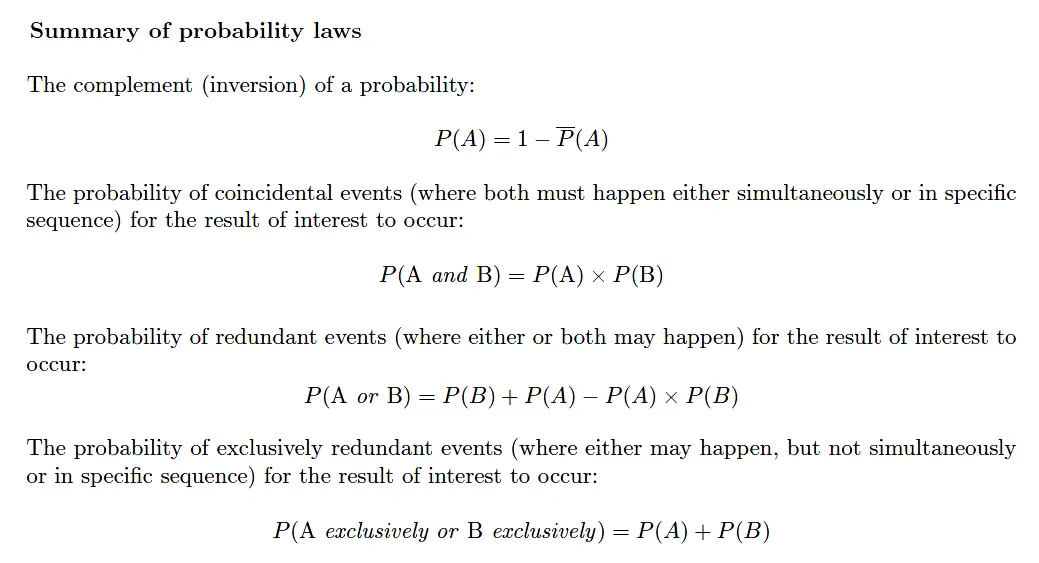
Given this similarity, we may apply standard Boolean operations such as NOT, AND, and OR to probabilities. These Boolean operations lead us to our first “laws” of probability for combination events.
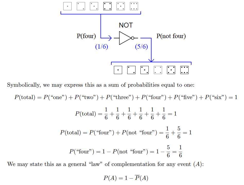
The logical “NOT” function
For instance, if we know the probability of rolling a “four” on a six-sided die is 1/6 , then we may safely say the probability of not rolling a “four” is 5/6 , the complement of 1/6 .
The common “inverter” logic symbol is shown here representing the complementation function, turning a probability of rolling a “four” into the probability of not rolling a “four”:
Complements of probability values find frequent use in reliability engineering. If we know the probability value for the failure of a component (i.e. how likely it is to fail when called upon to function – termed the Probability of Failure on Demand, or PFD – which is a measure of that component’s undependability), then we know the dependability value (i.e. how likely it is to function on demand) will be the mathematical complement.
To illustrate, consider a device with a PFD value of 1/100000 . Such a device could be said to have a dependability value of 99999/100000 , or 99.999%, since 1 − (1/100000) = 99999/100000 .
The logical “AND” function
The AND function regards probabilities of two or more coincidental events (i.e. where the outcome of interest only happens if two or more events happen together, or in a specific sequence).
Another example using a die is the probability of rolling a “four” on the first toss, then rolling a “one” on the second toss. It should be intuitively obvious that the probability of rolling this specific combination of values will be less (i.e. less likely) than rolling either of those values in a single toss.
The shaded field of possibilities (36 in all) demonstrate the unlikelihood of this sequential combination of values compared to the unlikelihood of either value on either toss:
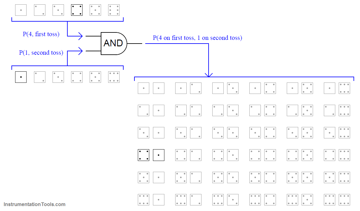
As you can see, there is only one outcome matching the specific criteria out of 36 total possible outcomes. This yields a probability value of one-in-thirty six ( 1/36 ) for the specified combination, which is the product of the individual probabilities. This, then, is our second law of probability:
P(A and B) = P(A) × P(B)
A practical application of this would be the calculation of failure probability for a double-block valve assembly, designed to positively stop the flow of a dangerous process fluid. Double-block valves are used to provide increased assurance of shut-off, since the shutting of either block valve is sufficient in itself to stop fluid flow.
The probability of failure for a double-block valve assembly – “failure” defined as not being able to stop fluid flow when needed – is the product of each valve’s un-dependability (i.e. probability of failing in the open position when commanded to shut off):
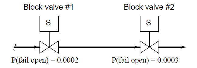
With these two valves in service, the probability of neither valve successfully shutting off flow (i.e. both valve 1 and valve 2 failing on demand; remaining open when they should shut) is the product of their individual failure probabilities.
P(assembly fail) = P(valve 1 fail open) × P(valve 2 fail open)
P(assembly fail) = 0.0002 × 0.0003
P(assembly fail) = 0.00000006 = 6 × 10⁻⁸
An extremely important assumption in performing such an AND calculation is that the probabilities of failure for each valve are completely unrelated.
For instance, if the failure probabilities of both valve 1 and valve 2 were largely based on the possibility of a certain residue accumulating inside the valve mechanism (causing the mechanism to freeze in the open position), and both valves were equally susceptible to this residue accumulation, there would be virtually no advantage to having double block valves.
If said residue were to accumulate in the piping, it would affect both valves practically the same. Thus, the failure of one valve due to this effect would virtually ensure the failure of the other valve as well.
The probability of simultaneous or sequential events being the product of the individual events’ probabilities is true if and only if the events in question are completely independent.
We may illustrate the same caveat with the sequential rolling of a die. Our previous calculation showed the probability of rolling a “four” on the first toss and a “one” on the second toss to be 1/6 × 1/6 , or 1/36 .
However, if the person throwing the die is extremely consistent in their throwing technique and the way they orient the die after each throw, such that rolling a “four” on one toss makes it very likely to roll a “one” on the next toss, the sequential events of a “four” followed by a “one” would be far more likely than if the two events were completely random and independent.
The probability calculation of 1/6 × 1/6 = 1/36 holds true only if all the throws’ results are completely unrelated to each other.
Another, similar application of the Boolean AND function to probability is the calculation of system reliability (R) based on the individual reliability values of components necessary for the system’s function.
If we know the reliability values for several essential system components, and we also know those reliability values are based on independent (unrelated) failure modes, the overall system reliability will be the product (Boolean AND) of those component reliabilities. This mathematical expression is known as Lusser’s product law of reliabilities:
Rsystem = R1 × R2 × R3 × · · · × Rn
As simple as this law is, it is surprisingly unintuitive. Lusser’s Law tells us that any system depending on the performance of several essential components will be less reliable than the leastreliable of those components. This is akin to saying that a chain will be weaker than its weakest link!
To give an illustrative example, suppose a complex system depended on the reliable operation of six key components in order to function, with the individual reliabilities of those six components being 91%, 92%, 96%, 95%, 93%, and 92%, respectively.
Given individual component reliabilities all greater than 90%, one might be inclined to think the overall reliability would be quite good. However, following Lusser’s Law we find the reliability of this system (as a whole) is only 65.3% because 0.91 × 0.92 × 0.96 × 0.95 × 0.93 × 0.92 = 0.653.
The logical “OR” function
The OR function regards probabilities of two or more redundant events (i.e. where the outcome of interest happens if any one of the events happen).
Another example using a die is the probability of rolling a “four” on the first toss or on the second toss. It should be intuitively obvious that the probability of rolling a “four” on either toss will be more probable (i.e. more likely) than rolling a “four” on a single toss.
The shaded field of possibilities (36 in all) demonstrate the likelihood of this either/or result compared to the likelihood of either value on either toss:
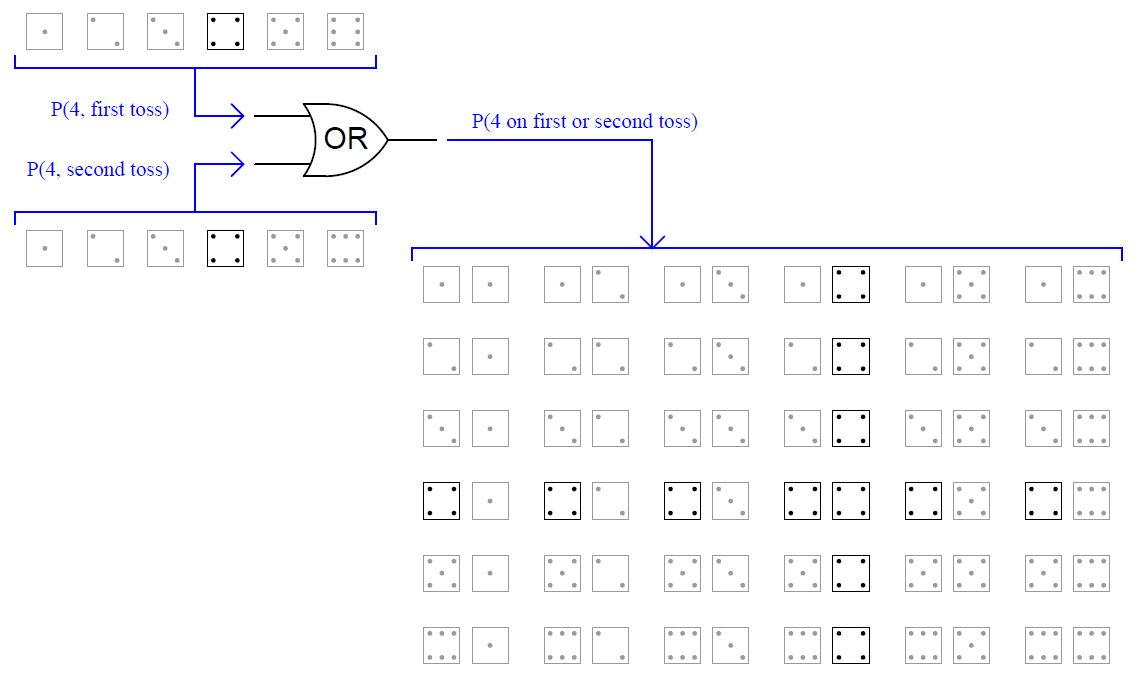
As you can see, there are eleven outcomes matching the specific criteria out of 36 total possible outcomes (the outcome with two “four” rolls counts as a single trial matching the stated criteria, just as all the other trials containing only one “four” roll count as single trials).
This yields a probability value of eleven-in-thirty six ( 11/36 ) for the specified combination. This result may defy your intuition, if you assumed the OR function would be the simple sum of individual probabilities ( 1/6 + 1/6 = 2/6 or 1/3 ), as opposed to the AND function’s product of probabilities ( 1/6 × 1/6 = 1/36 ).
In truth, there is an application of the OR function where the probability is the simple sum, but that will come later in this presentation.
As with the logical “AND” function, the logical “OR” function assumes the events in question are independent from each other. That is to say, the events lack a common cause, and are not contingent upon one another in any way.
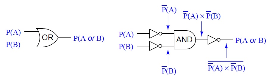
For now, a way to understand why we get a probability value of 11/36 for our OR function with two 1/6 input probabilities is to derive the OR function from other functions whose probability laws we already know with certainty.
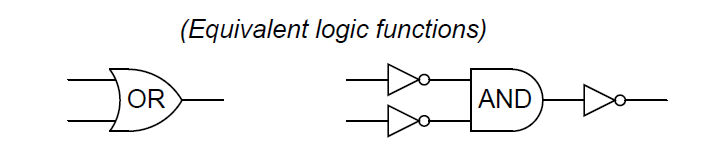
From Boolean algebra, DeMorgan’s Theorem tells us an OR function is equivalent to an AND function with all inputs and outputs inverted and the equation is
![]()
We already know the complement (inversion) of a probability is the value of that probability subtracted from one
![]()
This gives us a way to symbolically express the DeMorgan’s Theorem definition of an OR function in terms of an AND function with three inversions:
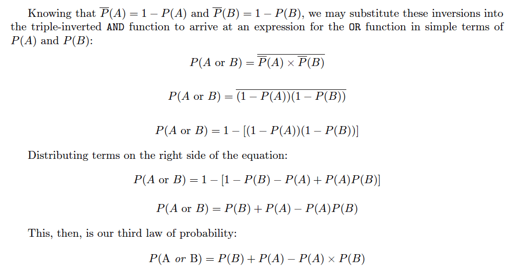
Inserting our example probabilities of 1/6 for both P(A) and P(B), we obtain the following probability for the OR function:

This confirms our previous conclusion of there being an 11/36 probability of rolling a “four” on the first or second rolls of a die.
We may return to our example of a double-block valve assembly for a practical application of OR probability. When illustrating the AND probability function, we focused on the probability of both block valves failing to shut off when needed, since both valve 1 and valve 2 would have to fail open in order for the double-block assembly to fail in shutting off flow.
Now, we will focus on the probability of either block valve failing to open when needed. While the AND scenario was an exploration of the system’s un-dependability (i.e. the probability it might fail to stop a dangerous condition), this scenario is an exploration of the system’s un-security (i.e. the probability it might fail to resume normal operation).
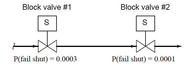
Each block valve is designed to be able to shut off flow independently, so that the flow of (potentially) dangerous process fluid will be halted if either or both valves shut off.
The probability that process fluid flow may be impeded by the failure of either valve to open is thus a simple (non-exclusive) OR function:
P(assembly fail) = P(valve 1 fail shut)+P(valve 2 fail shut)−P(valve 1 fail shut)×P(valve 2 fail shut)
P(assembly fail) = 0.0003 + 0.0001 − (0.0003 × 0.0001)
P(assembly fail) = 0.0003997 = 3.9997 × 10⁻⁴
A similar application of the OR function is seen when we are dealing with exclusive events. For instance, we could calculate the probability of rolling either a “three” or a “four” in a single toss of a die.
Unlike the previous example where we had two opportunities to roll a “four,” and two sequential rolls of “four” counted as a single successful trial, here we know with certainty that the die cannot land on “three” and “four” in the same roll.
Therefore, the exclusive OR probability (XOR) is much simpler to determine than a regular OR function:
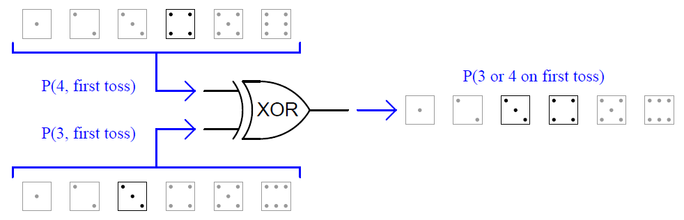
This is the only type of scenario where the function probability is the simple sum of the input probabilities.
In cases where the input probabilities are mutually exclusive (i.e. they cannot occur simultaneously or in a specific sequence), the probability of one or the other happening is the sum of the individual probabilities. This leads us to our fourth probability law:
P(A exclusively or B) = P(A) + P(B)
A practical example of the exclusive-or (XOR) probability function may be found in the failure analysis of a single block valve. If we consider the probability this valve may fail in either condition (stuck open or stuck shut), and we have data on the probabilities of the valve failing open and failing shut, we may use the XOR function to model the system’s general unreliability.
We know that the exclusive-or function is the appropriate one to use here because the two “input” scenarios (failing open versus failing shut) absolutely cannot occur at the same time:
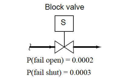
P(valve fail) = P(valve fail open) + P(valve fail shut)
P(valve fail) = 0.0002 + 0.0003
P(valve fail) = 0.0005 = 5 × 10⁻⁴
If the intended safety function of this block valve is to shut off the flow of fluid if a dangerous condition is detected, then the probability of this valve’s failure to shut when needed is a measure of its undependability.
Conversely, the probability of this valve’s failure to open under normal (safe) operating conditions is a measure of its unsecurity. The XOR of the valve’s undependability and its unsecurity therefore represents its unreliability.
The complement of this value will be the valve’s reliability: 1 − 0.0005 = 0.9995. This reliability value tells us we can expect the valve to operate as it’s called to 99.95% of the time, and we should expect 5 failures out of every 10,000 calls for action.


I am working with N-modular Redundant (HNMR) systems combine fault detection/recover means to achieve high level of fault tolerance and reliability.