Smart Transmitters LRV & URV

The advent of “smart” field instruments containing microprocessors has been a great advance for industrial instrumentation. These devices have built-in diagnostic ability, greater accuracy (due to digital compensation of sensor nonlinearities), and the ability to communicate digitally with host devices for reporting of various parameters.

A simplified block diagram of a “smart” pressure transmitter looks something like this:

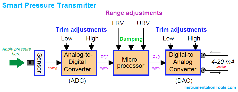
It is important to note all the adjustments within this device, and how this compares to the relative simplicity of an all-analog pressure transmitter:

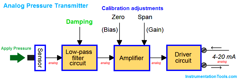
Note how the only calibration adjustments available in the analog transmitter are the “zero” and “span” settings. This is clearly not the case with smart transmitters. Not only can we set lower and upper-range values (LRV and URV) in a smart transmitter, but it is also possible to calibrate the analog-to-digital and digital-to-analog converter circuits independently of each other. What this means for the calibration technician is that a full calibration procedure on a smart transmitter potentially requires more work and a greater number of adjustments than an all-analog transmitter.

A common mistake made among students and experienced technicians alike is to confuse the range settings (LRV and URV) for actual calibration adjustments. Just because you digitally set the LRV of a pressure transmitter to 0.00 PSI and the URV to 100.00 PSI does not necessarily mean it will register accurately at points within that range! The following example will illustrate this fallacy.

Suppose we have a smart pressure transmitter ranged for 0 to 100 PSI with an analog output range of 4 to 20 mA, but this transmitter’s pressure sensor is fatigued from years of use such that an actual applied pressure of 100 PSI generates a signal that the analog-to-digital converter interprets as only 96 PSI. Assuming everything else in the transmitter is in perfect condition, with perfect calibration, the output signal will still be in error:

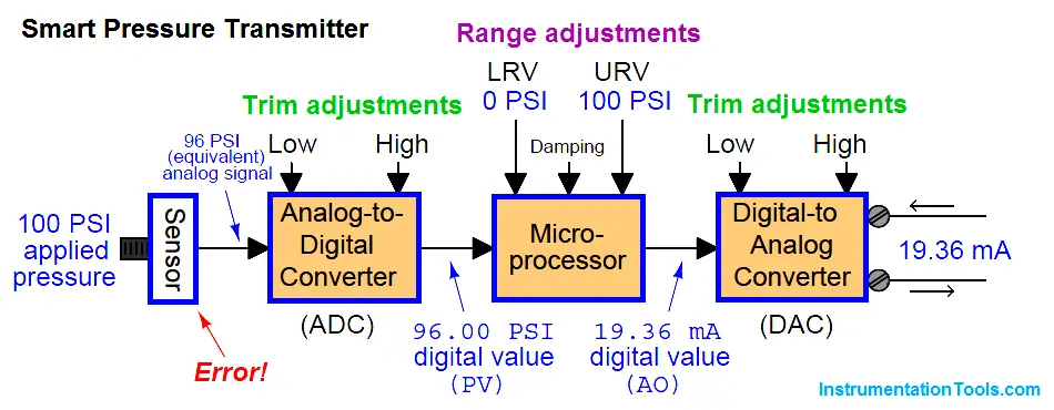
As the saying goes, “a chain is only as strong as its weakest link.” Here we see how the calibration of the most sophisticated pressure transmitter may be corrupted despite perfect calibration of both analog/digital converter circuits, and perfect range settings in the microprocessor. The microprocessor “thinks” the applied pressure is only 96 PSI, and it responds accordingly with a 19.36 mA output signal. The only way anyone would ever know this transmitter was inaccurate at 100 PSI is to actually apply a known value of 100 PSI fluid pressure to the sensor and note the incorrect response. The lesson here should be clear: digitally setting a smart instrument’s LRV and URV points does not constitute a legitimate calibration of the instrument.

For this reason, smart instruments always provide a means to perform what is called a digital trim on both the ADC and DAC circuits, to ensure the microprocessor “sees” the correct representation of the applied stimulus and to ensure the microprocessor’s output signal gets accurately converted into a DC current, respectively.

A convenient way to test a digital transmitter’s analog/digital converters is to monitor the microprocessor’s process variable (PV) and analog output (AO) registers while comparing the real input and output values against trusted calibration standards. A HART communicator device provides this “internal view” of the registers so we may see what the microprocessor “sees.” The following example shows a differential pressure transmitter with a sensor (analog-to-digital) calibration error:

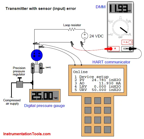
Here, the calibration standard for pressure input to the transmitter is a digital pressure gauge, registering 25.00 inches of water column. The digital multimeter (DMM) is our calibration standard for the current output, and it registers 11.93 milliamps. Since we would expect an output of 12.00 milliamps at this pressure (given the transmitter’s range values of 0 to 50 inches W.C.), we immediately know from the pressure gauge and multimeter readings that some sort of calibration error exists in this transmitter.

Comparing the HART communicator’s displays of PV and AO against our calibration standards reveals more information about the nature of this error: we see that the AO value (11.930 mA) agrees with the multimeter while the PV value (24.781 ”W.C.) does not agree with the digital pressure gauge. This tells us the calibration error lies within the sensor (input) of the transmitter and not with the DAC (output). Thus, the correct calibration procedure to perform on this errant transmitter is a sensor trim.

In this next example, we see what an output (DAC) error would look like with another differential pressure transmitter subjected to the same test:

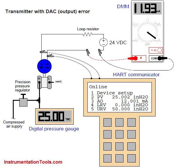
Once again, the calibration standard for pressure input to the transmitter is a digital pressure gauge, registering 25.00 inches of water column. A digital multimeter (DMM) still serves as our calibration standard for the current output, and it registers 11.93 milliamps. Since we expect 12.00 milliamps output at this pressure (given the transmitter’s range values of 0 to 50 inches W.C.), we immediately know from the pressure gauge and multimeter readings that some sort of calibration error exists in this transmitter (just as before).

Comparing the HART communicator’s displays of PV and AO against our calibration standards reveals more information about the nature of this error: we see that the PV value (25.002 inches W.C.) agrees with the digital pressure gauge while the AO value (12.001 mA) does not agree with the digital multimeter. This tells us the calibration error lies within the digital-to-analog converter (DAC) of the transmitter and not with the sensor (input). Thus, the correct calibration procedure to perform on this errant transmitter is an output trim.

Note how in both scenarios it was absolutely necessary to interrogate the transmitter’s microprocessor registers with a HART communicator to determine where the error was located. Merely comparing the pressure and current standards’ indications was not enough to tell us any more than the fact we had some sort of calibration error inside the transmitter. Not until we viewed the microprocessor’s own values of PV and AO could we determine whether the calibration error was related to the ADC (input), the DAC (output), or perhaps even both.

Sadly, I have witnessed technicians attempt to use the LRV and URV settings in a manner not unlike the zero and span adjustments on an analog transmitter to correct errors such as these. While it may be possible to get an out-of-calibration transmitter to yield correct output current signal values over its calibrated range of input values by skewing the LRV and URV settings, it defeats the purpose of having separate “trim” and “range” settings inside the transmitter.

Also, it causes confusion if ever the control system connected to the transmitter interrogates process variable values digitally rather than interpreting it via the 4-20 mA loop current signal. Finally, “calibrating” a transmitter by programming it with skewed LRV/URV settings corrupts the accuracy of any intentionally nonlinear functions such as square-root characterization (used for flow measurement applications) or strapping tables (used for liquid level measurement applications in vessels where the cross-sectional area varies with liquid height).

Once digital trims have been performed on both input and output converters, of course, the technician is free to re-range the microprocessor as many times as desired without re-calibration. This capability is particularly useful when re-ranging is desired for special conditions, such as process start-up and shut-down when certain process variables drift into uncommon regions. An instrument technician may use a hand-held HART communicator device to re-set the LRV and URV range values to whatever new values are desired by operations staff without having to re-check calibration by applying known physical stimuli to the instrument.

So long as the ADC and DAC trims are both correct, the overall accuracy of the instrument will still be good with the new range. With analog instruments, the only way to switch to a different measurement range was to change the zero and span adjustments, which necessitated the re-application of physical stimuli to the device (a full re-calibration). Here and here alone we see where calibration is not necessary for a smart instrument. If overall measurement accuracy must be verified, however, there is no substitute for an actual physical calibration, and this entails both ADC and DAC “trim” procedures for a smart instrument.

Completely digital (“Fieldbus”) transmitters are similar to “smart” analog-output transmitters with respect to distinct trim and range adjustments.