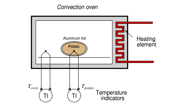
Simple, self-regulating processes tend to be first-order: that is, they have only one mechanism of lag. More complicated processes often consist of multiple sub-processes, each one with its own lag time. Take for example a convection oven, heating a potato. Being instrumentation specialists in addition to cooks, we decide to monitor both the oven temperature and the potato temperature using thermocouples and remote temperature indicators:
The oven itself is a first-order process. Given enough time and sufficiently thorough air circulation, the oven’s air temperature will eventually self-stabilize at the heating element’s temperature. If we graph its temperature over time as the heater power is suddenly stepped up to some fixed value (Note1) , we will see a classic first-order response:
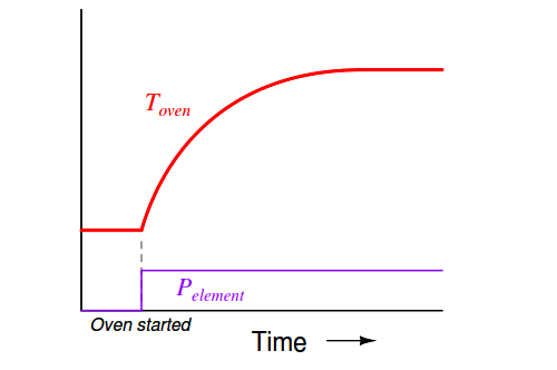
Note1 : We will assume here the heating element reaches its final temperature immediately upon the application of power, with no lag time of its own.
The potato forms another first-order process, absorbing heat from the air within the oven (heat transfer by convection), gradually warming up until its temperature (eventually) reaches that of the oven (Note1) . From the perspective of the heating element to the oven air temperature, we have a first-order process. From the perspective of the heating element to the potato, however, we have a second-order process.
Note 1 : Given the presence of water in the potato which turns to steam at 212 deg F, things are just a bit more complicated than this, but let’s ignote the effects of water in the potato for now!
Intuition might lead you to believe that a second-order process is just like a first-order process – except slower – but that intuition would be wrong. Cascading two first-order lags creates a fundamentally different time dynamic. In other words, two first-order lags do not simply result in a longer first-order lag, but rather a second-order lag with its own unique characteristics.
If we superimpose a graph of the potato temperature with a graph of the oven temperature (once again assuming constant power output from the heating element, with no thermostatic control), we will see that the shape of this second-order lag is different. The curve now has an “S” shape, rather than a consistent downward concavity:
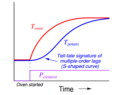
This, in fact, is one of the tell-tale signature of multiple lags in a process: an “S”-shaped curve rather than the characteristically abrupt initial rise of a first-order curve.
Another tell-tale signature of multiple lags is that the lagging variable does not immediately reverse its direction of change following a reversal in the final control element signal. We can see this effect by cutting power to the heating element before either the oven air or potato temperatures have reached their final values:
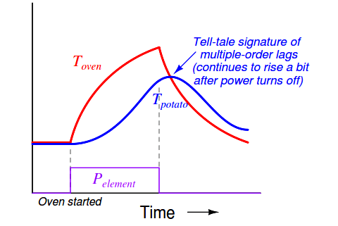
Note how the air temperature trend immediately reverses direction following the cessation of power to the heating element, but how the potato temperature trend continues to rise for a short amount of time (Note2) before reversing direction and cooling. Here, the contrast between first-order and second-order lag responses is rather dramatic – the second-order response is clearly not just a longer version of the first-order response, but rather something quite distinct unto itself.
Note 2 : The amount of time the potato’s temperature will continue to rise following the down-step in heating element power is equal to the time it takes for the oven’s air temperature to equal the potato’s temperature. The reason the potato’s temperature keeps rising after the heating element turns off is because the air inside the oven is (for a short time) still hotter than the potato, and therefore the potato continues to absorb thermal energy from the air for a time following power-off.
This is why multiple-order lag processes have a greater tendency to overshoot their setpoints while under automatic control: the process variable exhibits a sort of “inertia” whereby it fails to switch directions simultaneously with the controller output.
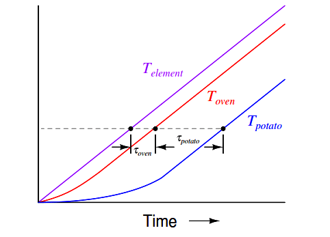
If we were able to ramp the heater power at a constant rate and graph the heater element, air, and potato temperatures, we would clearly see the separate lag times of the oven and the potato as offsets in time at any given temperature:
As another example, let us consider the control of level in three cascaded, gravity-drained vessels:
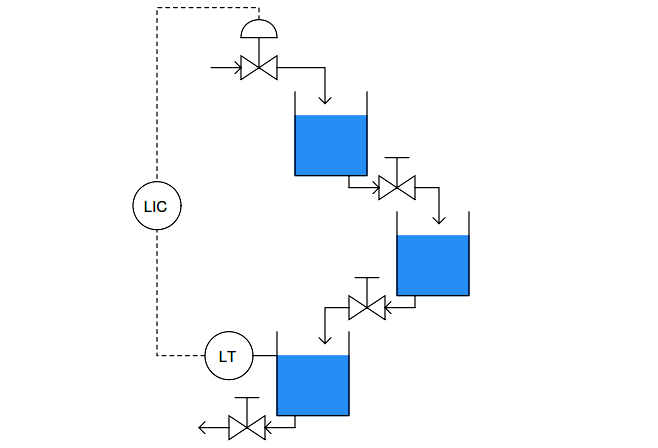
From the perspective of the level transmitter on the last vessel, the control valve is driving a third-order process, with three distinct lags cascaded in series. This would be a challenging process to control, and not just because of the possibility of the intermediate vessels overflowing (since their levels are not being measured)!
When we consider the dynamic response of a process, we are usually concerned primarily with the physical process itself. However, the instruments attached to that process also influence lag orders and lag times. As discussed in the previous subsection, almost every physical function exhibits some form of lag. Even the instruments we use to measure process variables have their own (usually very short) lag times. Control valves may have substantial lag times, measured in the tens of seconds for some large valves. Thus, a “slow” control valve exerting control over a first-order process effectively creates a second-order loop response. Thermowells used with temperature sensors such as thermocouples and RTDs can also introduce lag times into a loop (especially if the sensing element is not fully contacting the bottom of the well!).
This means it is nearly impossible to have a control loop with a purely first-order response. Many real loops come close to being first-order, but only because the lag time of the physical process swamps (dominates) the relatively tiny lag times of the instruments. For inherently fast processes such as liquid flow and liquid pressure control, however, the process response is so fast that even short time lags in valve positioners, transmitters, and other loop instruments significantly alter the loop’s dynamic character.
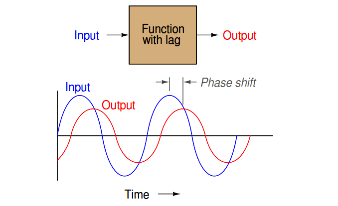
Multiple-order lags are relevant to the issue of PID loop tuning because they encourage oscillation. The more lags there are in a system, the more delayed and “detached” the process variable becomes from the controller’s output signal. A system with lag time exhibits phase shift when driven by a sinusoidal stimulus: the outgoing waveform lags behind the input waveform by a certain number of degrees at one frequency. The exact amount of phase shift depends on frequency – the higher the frequency, the more phase shift (to a maximum of −90 degc for a first-order lag):
The phase shifts of multiple, cascaded lag functions (or processes, or physical effects) add up. This means each lag in a system contributes an additional negative phase shift to the loop. This can be detrimental to negative feedback, which by definition is a 180 deg phase shift. If sufficient lags exist in a system, the total loop phase shift may approach 360 deg, in which case the feedback becomes positive (regenerative): a necessary condition for oscillation.
It is worthy to note that multiple-order lags are constructively applied in electronics when the express goal is to create oscillations. If a series of RC “lag” networks are used to feed the output of an inverting amplifier circuit back to its input with sufficient signal strength intact , and those networks introduce another 180 degrees of phase shift, the total loop phase shift will be 360 deg (i.e. positive feedback) and the circuit will self-oscillate. This is called an RC phase-shift oscillator circuit:
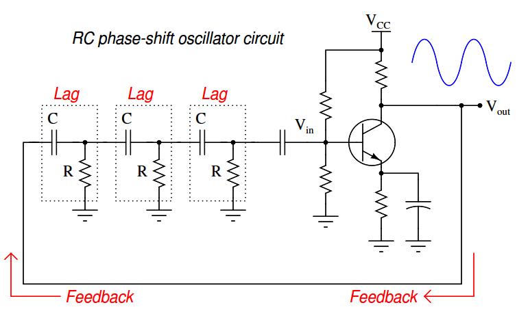
The amplifier works just like a proportional-only process controller, with action set for negative feedback. The resistor-capacitor networks act like the lags inherent to the process being controlled. Given enough controller (amplifier) gain, the cascaded lags in the process (RC networks) create the perfect conditions for self-oscillation. The amplifier creates the first 180 deg of phase shift (being inverting in nature), while the RC networks collectively create the other 180 deg of phase shift to give a total phase shift of 360 deg (positive, or regenerative feedback).
In theory, the most phase shift a single RC network can create is −90 deg , but even that is not practical. This is why more than two RC phase-shifting networks are required for successful operation of an RC phase-shift oscillator circuit.