Unlike the discrete/digital (on/off) circuit, analog signals vary across a range of voltage or current. Taking the same vessel described previously in Digital wiring example, how would the wiring change if we replaced the switch with a level transmitter?
PLC Analog Signals Wiring Techniques
The below Figure has the same circuit-breaker panel, but now it is feeding a DC power supply.
The power supply could be in its own cabinet, or it could be in the marshalling panel. In any case, DC power is distributed in the marshalling panel. A single fuse could power several circuits, or each circuit could be fused.

The transmitter is fed +24 VDC at its positive terminal. The 4–20 mA current signal is sourced from the (-) terminal of the transmitter to the PLC.
Cabling is twisted pair and shielded. The signal cable is numbered with the transmitter number, and the wires inside are numbered to provide power source information.
The shield is terminated in the marshalling panel, where all shields are gathered and terminated to a ground lug that is isolated from the cabinet. Note: Care should be used to ensure that the shield is only grounded at one spot.
Shields that are grounded in more than one spot may inject large noise spikes onto the signal. This condition is called a ground loop and can be a very difficult problem to isolate, as the problem is intermittent.
A “quiet” ground should be used to ground all the shields at one point. A quiet ground is one that is either tied to a dedicated ground triad, or one that is tied to the center-tap of an isolation transformer.
Noisy ground would be one that is physically located far from the transformer, and one that services motors, lights, or other noisy items. That is the basic two-wire analog input circuit.
The following is some specific information regarding the various analog possibilities:
a. Circuit Protection (Fusing)
Analog circuits are always low voltage, usually 24 VDC. As a result, fusing individual analog circuits is not required for personnel safety. Also, most analog I/O modules have current-limiting circuits onboard.
So fusing is generally not required to protect the modules. If these two conditions are true—and the designer should confirm this with the manufacturer— then per-point fusing can be avoided if desired.
If a designer wishes to save money by not fusing every point, then grouping the circuits into damage control zones should be considered.
For example, if there is a pump pair, a primary and a backup, instruments for the two should be in separate fuse groups to prevent a single blown fuse from taking them both out. For more information, see I/O Partitioning in the index.
b. Noise Immunity
Analog circuits are susceptible to electronic noise. If, for example, an analog cable lies adjacent to a motor’s high-voltage cable, then the analog signal cable will act as an antenna, picking up the magnetically coupled noise generated by the motor.
Other sources of noise exist, such as radio frequency (RF) radiation from a walkie-talkie. Noise on an analog signal cable can cause errors in reading the value of the signal, which in turn can cause a multitude of problems in the control system.
Some ways to mitigate noise include:
• Twisted-Pair Cables:
Electronic noise may be greatly reduced by the use of twisted-pair cabling. Most instruments use two wires to transmit their signals. Current flows out to the device in one wire and back from the device in the other.
If these wires are twisted, then the noise induced will be very nearly the same in each wire.
The magnitude of induced current flow is identical in each conductor, but it travels in opposite directions, thus canceling out most of the noise.
• Shielding:
A further refinement in noise rejection is shielding, i.e., the use of a grounded braid or foil shield around the conductors. As previously mentioned, the shield should never be grounded in more than one place to avoid ground loops.
Most instrument manufacturers recommend grounding the shield at the field instrument. However, a better place to do it is in the marshalling panel.
It is easier to verify and manage the grounds if they are in one place. Also, it is possible to ensure a good ground at that point.
• Conduit:
A final refinement in noise rejection is grounded metallic conduit. This is rarely required, except for data communications cables and for particularly critical circuits.
c. Resistance Temperature Detector (RTD)
An RTD is made of a special piece of wire whose electrical resistance changes in a predictable way when the wire is exposed to varying temperatures.
The material of choice today is 100 ohm platinum, though other types, such as 10 ohm copper, are sometimes used. For the platinum RTD, the rating is for 100 ohms at 0ºC.
Resistance changes with temperature are very small, causing voltage variations in the millivolt range.
RTDs are connected to a Wheatstone bridge circuit that is tuned to the RTD. But this tuning occurs on the bench.
What about the field environment? We have already discussed the line attenuation difficulties inherent in millivolt signals (Chapter 4). This problem is overcome in the RTD circuit by the use of one or two sense inputs.
These inputs help negate the effects of copper losses due to long lines and temperature variations along them and are additional wires that must be included in the RTD cable, hence the terms three-wire and four-wire RTDs.
d. Thermocouple
As we have discussed, a thermocouple exploits the electromotive force (EMF) that arises from changes in temperature affecting two dissimilar metals that have been laminated together.
This EMF manifests itself as a millivolt (DC) signal. When certain combinations of these dissimilar metals are joined, a predictable curve of temperature to voltage results as temperature at the junction changes.
The signal is measured at the open end of the two wires, and a millivolt-per-degree scale is used to convert the voltage to engineering units.
Thermocouple is thus a two-wire device. It is susceptible to radiated and induced noise and so is usually housed in a shielded cable if extended for a very long distance. The thermocouple signal is also susceptible to degradation due to line loss, so minimizing the cable length is desirable.
Also, it is important to use the proper extension wire. A thermocouple usually comes with a short pigtail connection to which extension wire must be attached. If a different wire material, such as copper, is used to extend the signal to the PLC, a spurious “cold junction” is created that causes a reverse EMF that partially cancels out the signal.
Therefore, the proper extension wire should be used, or a device called a cold-junction compensator or ice-point reference needs to be installed between the copper wiring and the thermocouple wiring.
Thermocouple I/O modules already have the cold-junction compensation onboard, so using the proper thermocouple extension wire is required.
Specific types of thermocouples exhibit different temperature characteristics. A type J thermocouple is formed by joining an iron wire with a constantan wire.
This configuration provides a curve relatively linear between 0 and 750ºC.8 A type K thermocouple has a nickel-chromium wire mated to a nickel-aluminum wire, sometimes called chromel/alumel.
The type K thermocouple spans a useful temperature range of -200 to 1250ºC. Other combinations yield different response curves.
e. 0–10 Millivolt (mV) Analog
Analog signals were first generated by voltage modulation. In the old days, a transmitter would generate a weak signal that had to be captured and then filtered and amplified so it could be used to move a pen on a recorder, or a needle on a gauge. The Achilles’ heel of the millivolt signal is its susceptibility to electrical noise.
This signal-to-noise ratio problem increases as a function of cable length. So the transmitter needed to be in close proximity to the indicator or recorder.
Millivolt signals today are, by and large, fed to transducers that convert the small signal to a current or to other media (like digital data values) less susceptible to noise and decibel (dB) loss before leaving the vicinity of the sensing element. However, some recorders and data acquisition systems still operate on the millivolt signal.
f. 4–20 Milliamp (mA) Analog
The drive to overcome the line attenuation shortcomings of the millivolt signal resulted in the development of the 4–20 mA current loop.
As a result of its greatly increased performance, this method of transmitting analog signals quickly became the industry standard. Most field instruments on the market have a sensing element (sensor) and a transmitting element.
The transmitter is tuned to the sensor, which may provide any type of signal from frequency-modulated analog to millivolts DC.
Whatever the form of the signal, the transmitter interprets it and converts it to an output current between 4 and 20 mA and within that span is proportional in magnitude to the input. The process of tuning the output to the input is called scaling.
Thus, the transmitter becomes what is referred to as a variable-current source. Just as a battery, as a voltage source, tries to maintain a constant voltage, regardless of the amount of load applied to it, the current source tries to maintain a constant current (for a given input signal), regardless of load.
Since current is common at all points of a series circuit, the problem of cable length—as noted as a problem with the millivolt signal—is nullified.
Of course, the ability of the device to force a constant current through a circuit can be overcome if enough load is applied. Therefore, the designer must know how much energy the current source is capable of producing.
Generally, today’s instruments are able to maintain 20 mA at a circuit resistance of 1000 ohms. Since a typical instrument has no more than 250 ohms of input resistance, it is possible to power several instruments from a single current source without needing an isolator.
For example, a single transmitter should be able to feed its signal to a PLC, a chart recorder, and a totalizer at a cost of 750 ohms, plus the line resistance. This should still be within the comfort zone of a typical transmitter.
Note: There are still instruments with 600 ohm ratings on the market, so the designer should always check whenever a complex circuit is contemplated.
To determine the energy available to the circuit, the designer must be able to identify the provider of that energy. That task is sometimes not as straightforward as it might appear, and the answer to the question will greatly impact the wiring of the circuit.
There are two primary types of analog circuit, as described from the point of view of the transmitter. Transmitters with two wires are considered to be passive devices that sink current, while transmitters with four wires are active devices that source current.
The below Figure depicts three temperature transmitters, each connected to different I/O points on the same PLC module.
One transmitter is directly powered (i.e., four-wire), while the others are indirectly powered (i.e., two-wire). Each transmitter is connected to a control device—in this case, a PLC input.
From the PLC’s perspective, all 4–20 mA current inputs are really voltage inputs. Resistors, either user-provided external ones, as shown here, or internal ones, are used to convert the current to a voltage.
The computer points themselves are actually high-resistance voltmeters, which give them excellent isolation from the field devices and minimize additional loading on the input circuit.
The I/O points on the PLC are shown with internal power available for each point, so the module is capable of being the voltage source for the loop.

The following is a detailed commentary on the differences between two-wire and four-wire devices:
1. Four-Wire Circuit
As seen below, a four-wire transmitter is one that provides the energy to power the loop and generate the current-modulated signal.
Most level transmitters, for example, are four-wire devices. Four-wire devices always have power connections in addition to the signal connections. Yet not all such powered transmitters are four-wire.
If a powered transmitter’s output is noted as passive, then the device may be treated as a two-wire unit from the standpoint of the signal circuit.
Most recording devices are externally powered, but are passive on the circuit. In these cases, the external power is for the internal electronics of the unit only.
The signal circuit is isolated from this power source. Note that the recorder shown on the bottom circuit is a powered, passive device.
2. Two-Wire Circuit
A two-wire device is said to be loop powered. This means the device functions by absorbing the energy it needs to generate the signal from the current loop.
This is also referred to as “current sinking.” This nomenclature can be a bit confusing because a transmitter that is current sinking is still the signal source for the circuit. Power for the current loop is supplied elsewhere.
A transmitter classified as two-wire must typically be the first device in the circuit with respect to current flow.
In other words, the positive terminal of the transmitter must be directly connected to the positive terminal of the voltage source. The voltage source is usually a 24 VDC power supply.
(a) Two-Wire Circuits with Stand-Alone Power Supply
Referring to above Figure, PLC I/O point 2 depicts a two-wire circuit with an external DC power supply.
Notice the wires must be rolled (polarity-wise) at the PLC for the proper polarity to be present across the I/O point.
That is because current flow is now reversed with respect to the previous example because the transmitter must become the first load in the loop as opposed to being the energy source for the loop.
(b) Two-Wire Circuits with PLC Internal Power Supply
Most PLC systems today are able to source the loop current themselves by simply connecting the positive terminal of the transmitter to a different terminal at the PLC.
The negative terminal of the transmitter is then tied to the positive side of the I/O point, and the negative side of the I/O point is jumpered to the PLC system’s DC common.
That is depicted in the I/O point 3 example. In that example, a recorder has been added to the loop.
If you liked this article, then please subscribe to our YouTube Channel for PLC and SCADA video tutorials.
You can also follow us on Facebook and Twitter to receive daily updates.
Read Next:
4-wire Passive vs Active Transmitters
PLC SCADA Engineers Interview Questions


Really informative!!! Keep it up bro!
This is the Best Site for the people who belongs to INSTRUMENTATION,AUTOMATION,CONTROL field. I love this Site and If anyone who follows only this single site can become the Master of this Field.
Mr. S Bharadwaj Reddy is doing highly appreciable job by providing Technical articles.
why we use this type of conection in fig2 section 2 and what is R and ..?
i undrestand with a look at the direction of current
excellent thanks reddy ..?
thanks
Useful info
Comment diagnostiquer un thermocouple et un transmetteur de pression 4-20 mA avec un mutlimettre ?
For 4wire Analog Input, need fuse blown indication for 4-20 mA