Integral (Reset) Control Theory

Imagine a liquid-level control system for a vessel, where the position of a level-sensing float sets the position of a potentiometer, which then sets the speed of a motor-actuated control valve. If the liquid level is above setpoint, the valve continually opens up; if below setpoint, the valve continually closes off:

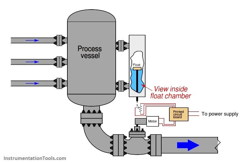
Unlike the proportional control system where valve position was a direct function of float position, this control system sets the speed of the motor-driven valve according to the float position. The further away from setpoint the liquid level is, the faster the valve moves open or closed. In fact, the only time the valve will ever halt its motion is when the liquid level is precisely at setpoint; otherwise, the control valve will be in constant motion.

This control system does its job in a very different manner than the all-mechanical float-based proportional control system illustrated previously. Both systems are capable of regulating liquid level inside the vessel, but they take very different approaches to doing so. One of the most significant differences in control behavior is how the proportional system would inevitably suffer from offset (a persistent error between PV and SP), whereas this control system actively works at all times to eliminate offset. The motor-driven control valve literally does not rest until all error has been eliminated!

Instead of characterizing this control system as proportional, we call it integral in honor of the calculus principle (“integration”) whereby small quantities are accumulated over some span to form a total. Don’t let the word “calculus” scare you! You are probably already familiar with the concept of numerical integration even though you may have never heard of the term before.

Calculus is a form of mathematics dealing with changing variables, and how rates of change relate between different variables. When we “integrate” a variable with respect to time, what we are doing is accumulating that variable’s value as time progresses. Perhaps the simplest example of this is a vehicle odometer, accumulating the total distance traveled by the vehicle over a certain time period. This stands in contrast to a speedometer, indicating the rate of distance traveled per unit of time.

Imagine a car moving along at exactly 30 miles per hour. How far will this vehicle travel after 1 hour of driving this speed? Obviously, it will travel 30 miles. Now, how far will this vehicle travel if it continues for another 2 hours at the exact same speed? Obviously, it will travel 60 more miles, for a total distance of 90 miles since it began moving. If the car’s speed is a constant, calculating total distance traveled is a simple matter of multiplying that speed by the travel time.

The odometer mechanism that keeps track of the mileage traveled by the car may be thought of as integrating the speed of the car with respect to time. In essence, it is multiplying speed times time continuously to keep a running total of how far the car has gone. When the car is traveling at a high speed, the odometer “integrates” at a faster rate. When the car is traveling slowly, the odometer “integrates” slowly.

If the car travels in reverse, the odometer will decrement (count down) rather than increment (count up) because it sees a negative quantity for speed. The rate at which the odometer decrements depends on how fast the car travels in reverse. When the car is stopped (zero speed), the odometer holds its reading and neither increments nor decrements.

Now let us return to the context of an automated process to see how this calculus principle works inside a process controller. Integration is provided either by a pneumatic mechanism, an electronic opamp circuit, or by a microprocessor executing a digital integration algorithm. The variable being integrated is error (the difference between PV and SP) over time. Thus the integral mode of the controller ramps the output either up or down over time in response to the amount of error existing between PV and SP, and the sign of that error. We saw this “ramping” action in the behavior of the liquid level control system using a motor-driven control valve commanded by a float-positioned potentiometer: the valve stem continuously moves so long as the liquid level deviates from setpoint. The reason for this ramping action is to increase or decrease the output as far as it is necessary in order to completely eliminate any error and force the process variable to precisely equal setpoint. Unlike proportional action, which simply moves the output an amount proportional to any change in PV or SP, integral control action never stops moving the output until all error is eliminated.

If proportional action is defined by the error telling the output how far to move, integral action is defined by the error telling the output how fast to move. One might think of integral as being how “impatient” the controller is, with integral action constantly ramping the output as far as it needs to go in order to eliminate error. Once the error is zero (PV = SP), of course, the integral action stops ramping, leaving the controller output (valve position) at its last value just like a stopped car’s odometer holds a constant value. If we add an integral term to the controller equation, we get something that looks like this :

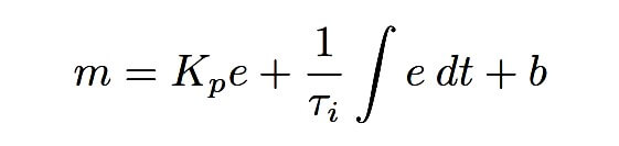
Where,
m = Controller output
e = Error (difference between PV and SP)
Kp = Proportional gain
Ti = Integral time constant (minutes)
t = Time
b = Bias

The most confusing portion of this equation for those new to calculus is the part that says “ ∫ e dt”. The integration symbol (looks like an elongated letter “S”) tells us the controller will accumulate (“sum”) multiple products of error (e) over tiny slices of time (dt). Quite literally, the controller multiplies error by time (for very short segments of time, dt) and continuously adds up all those products to contribute to the output signal which then drives the control valve (or other final control element). The integral time constant (Ti ) is a value set by the technician or engineer configuring the controller, proportioning this cumulative action to make it more or less aggressive over time.

To see how this works in a practical sense, let’s imagine how a proportional + integral controller would respond to the scenario of a heat exchanger whose inlet temperature suddenly dropped. As we saw with proportional-only control, an inevitable offset occurs between PV and SP with changes in load, because an error must develop if the controller is to generate the different output signal value necessary to halt further change in PV. We called this effect proportional-only offset.

Once this error develops, though, integral action begins to work. Over time, a larger and larger quantity accumulates in the integral mechanism (or register) of the controller due to the persistent error between PV and SP. That accumulated value adds to the controller’s output, driving the steam control valve further and further open. This, of course, adds heat at a faster rate to the heat exchanger, which causes the outlet temperature to rise. As the temperature re-approaches setpoint, the error becomes smaller and thus the integral action proceeds at a slower rate (like a car’s odometer incrementing at a slower rate as the car’s speed decreases).

So long as the PV is below SP (the outlet temperature is still too cool), the controller will continue to integrate upwards, driving the control valve further and further open. Only when the PV rises to exactly meet SP does integral action finally rest, holding the valve at a steady position. Integral action tirelessly works to eliminate any offset between PV and SP, thus neatly eliminating the offset problem experienced with proportional-only control action.

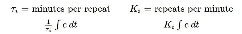
As with proportional action, there are (unfortunately) two completely opposite ways to specify the degree of integral action offered by a controller. One way is to specify integral action in terms of minutes or minutes per repeat. A large value of “minutes” for a controller’s integral action means a less aggressive integral action over time, just as a large value for proportional band means a less aggressive proportional action. The other way to specify integral action is the inverse: how many repeats per minute, equivalent to specifying proportional action in terms of gain (large value means aggressive action). For this reason, you will sometimes see the integral term of a PID equation written differently:

Many modern digital electronic controllers allow the user to select the unit they wish to use for integral action, just as they allow a choice between specifying proportional action as gain or as proportional band.

Integral is a highly effective mode of process control. In fact, some processes respond so well to integral controller action that it is possible to operate the control loop on integral action alone, without proportional. Typically, though, process controllers implement some form of proportional plus integral (“PI”) control.

Just as too much proportional gain will cause a process control system to oscillate, too much integral action (i.e. an integral time constant that is too short) will also cause oscillation. If the integration happens at too fast a rate, the controller’s output will “saturate” either high or low before the process variable can make it back to setpoint. Once this happens, the only condition that will “unwind” the accumulated integral quantity is for an error to develop of the opposite sign, and remain that way long enough for a canceling quantity to accumulate. Thus, the PV must cross over the SP, guaranteeing at least another half-cycle of oscillation.

A similar problem called reset windup (or integral windup) happens when external conditions make it impossible for the controller to achieve setpoint. Imagine what would happen in the heat exchanger system if the steam boiler suddenly stopped producing steam. As outlet temperature dropped, the controller’s proportional action would open up the control valve in a futile effort to raise temperature. If and when steam service is restored, proportional action would just move the valve back to its original position as the process variable returned to its original value (before the boiler died). This is how a proportional-only controller would respond to a steam “outage”: nice and predictably. If the controller had integral action, however, a much worse condition would result.

All the time spent with the outlet temperature below setpoint causes the controller’s integral term to “wind up” in a futile attempt to admit more steam to the heat exchanger. This accumulated quantity can only be un-done by the process variable rising above setpoint for an equal error-time product , which means when the steam supply resumes, the temperature will rise well above setpoint until the integral action finally “unwinds” and brings the control valve back to a same position again.

Various techniques exist to manage integral windup. Controllers may be built with limits to restrict how far the integral term can accumulate under adverse conditions. In some controllers, integral action may be turned off completely if the error exceeds a certain value. The surest fix for integral windup is human operator intervention, by placing the controller in manual mode. This typically resets the integral accumulator to a value of zero and loads a new value into the bias term of the equation to set the valve position wherever the operator decides. Operators usually wait until the process variable has returned at or near setpoint before releasing the controller into automatic mode again.

While it might appear that operator intervention is again a problem to be avoided (as it was in the case of having to correct for proportional-only offset), it is noteworthy to consider that the conditions leading to integral windup usually occur only during shut-down conditions. It is customary for human operators to run the process manually anyway during a shutdown, and so the switch to manual mode is something they would do anyway and the potential problem of windup often never manifests itself.

Integral control action has the unfortunate tendency to create loop oscillations (“cycling”) if the final control element exhibits hysteresis, such as the case with a “sticky” control valve. Imagine for a moment our steam-heated heat exchanger system where the steam control valve possesses excessive packing friction and therefore refuses to move until the applied air pressure changes far enough to overcome that friction, at which point the valve “jumps” to a new position and then “sticks” in that new position. If the valve happens to stick at a stem position resulting in the product temperature settling slightly below setpoint, the controller’s integral action will continually increase the output signal going to the valve in an effort to correct this error (as it should).

However, when that output signal has risen far enough to overcome valve friction and move the stem further open, it is very likely the stem will once again “stick” but this time do so at a position making the product temperature settle above setpoint. The controller’s integral action will then ramp downward in an effort to correct this new error, but due to the valve’s friction making precise positioning impossible, the controller can never achieve setpoint and therefore it cyclically “hunts” above and below setpoint.

The best solution to this “reset cycling” phenomenon, of course, is to correct the hysteresis in the final control element. Eliminating friction in the control valve will permit precise positioning and allow the controller’s integral action to achieve setpoint as designed. Since it is practically impossible to eliminate all friction from a control valve, however, other solutions to this problem exist.

One of them is to program the controller to stop integrating whenever the error is less than some pre-configured value (sometimes referred to as the “integral deadband” or “reset deadband” of the controller). By activating reset control action only for significant error values, the controller ignores small errors rather than “compulsively” trying to correct for any detected error no matter how small.