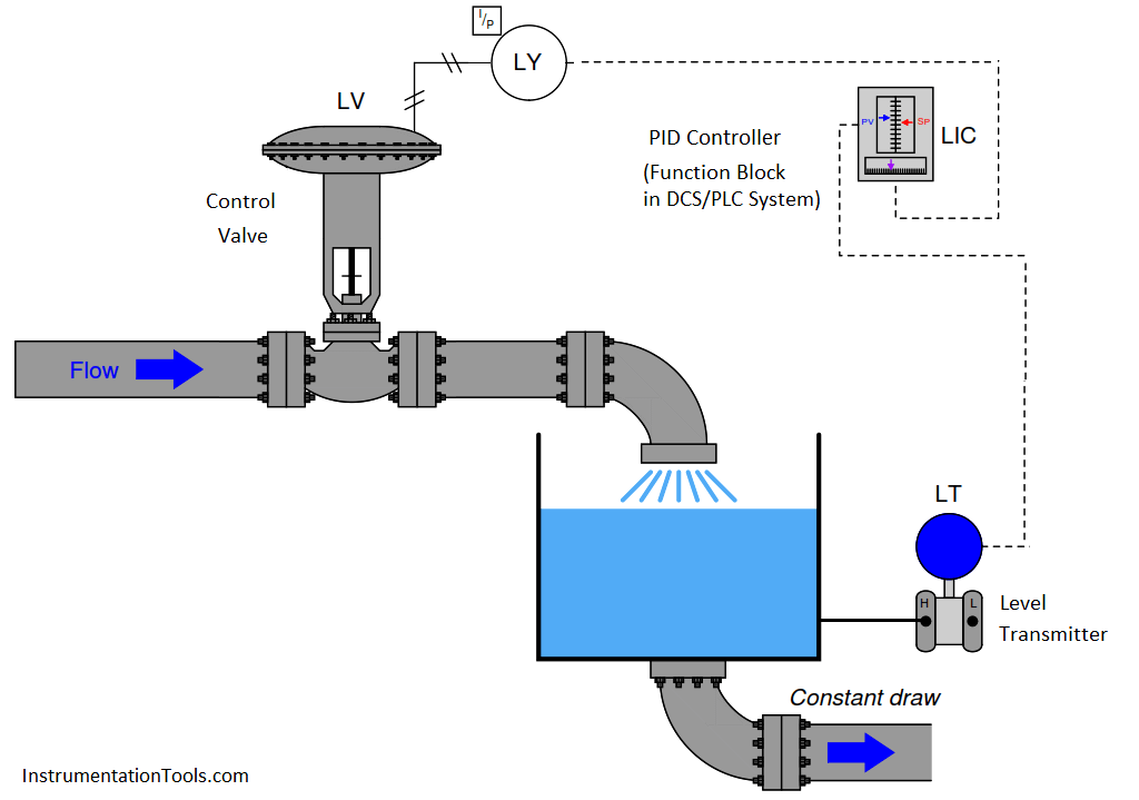
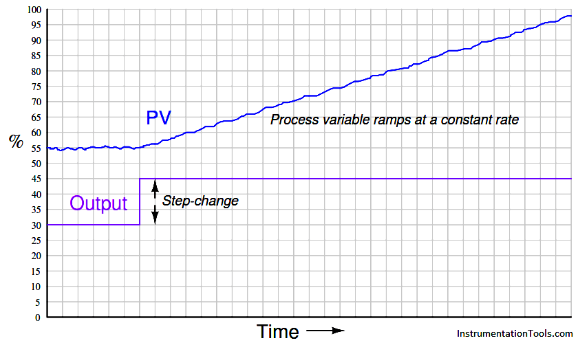
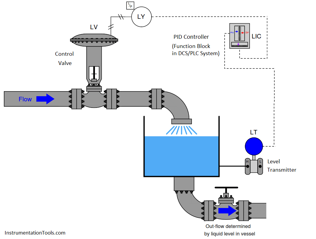
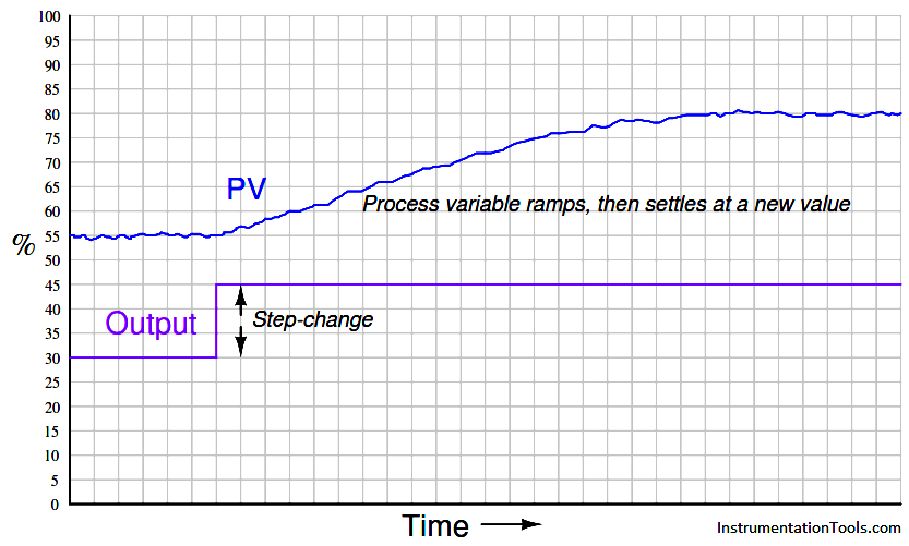
A good example of an integrating process is liquid level control, where either the flow rate of liquid into or out of a vessel is constant and the other flow rate varies. If a control valve is opened in a step-change fashion, liquid level in the vessel ramps at a rate proportional to the difference in flow rates in and out of the vessel. The following illustration shows a typical liquid level-control installation, with a process trend showing the level response to a step-change in valve position (with the controller in manual mode, for an “open-loop” test):
It is critically important to realize that this ramping action of the process variable over time is a characteristic of the process itself, not the controller. When liquid flow rates in and out of a vessel are mis-matched, the liquid level within that vessel will change at a rate proportional to the difference in flow rates. The trend shown here reveals a fundamental characteristic of the process, not the controller (this should be obvious once it is realized that the step-change in output is something that would only ever happen with the controller in manual mode). Mathematically, we may express the integrating nature of this process using calculus notation. First, we may express the rate of change of volume in the tank over time ( dV/dt ) in terms of the flow rates in and out of the vessel:
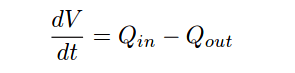
For example, if the flow rate of liquid going into the vessel was 450 gallons per minute, and the constant flow rate drawn out of the vessel was 380 gallons per minute, the volume of liquid contained within the vessel would increase over time at a rate equal to 70 gallons per minute: the difference between the in-flow and the out-flow rates.
Another way to express this mathematical relationship between flow rates and liquid volume in the vessel is to use the calculus function of integration:
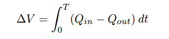
The amount of liquid volume accumulated in the vessel (∆V ) between time 0 and time T is equal to the sum (∫) of the products (multiplication) of difference in flow rates in and out of the vessel (Qin − Qout) during infinitesimal increments of time (dt).
In the given scenario of a liquid level control system where the out-going flow is held constant, this means the level will be stable only at one in-coming flow rate (where Q in = Qout ). At any other controlled flow rate, the level will either be increasing over time or decreasing over time.
This process characteristic perfectly matches the characteristic of a proportional-only controller, where there is one unique output value when the error is zero (PV = SP). We may illustrate this by performing a “thought experiment” on the liquid level-control process shown earlier having a constant draw out the bottom of the vessel. Imagine this process controlled by a proportional-only controller in automatic mode, with the bias value (b) of the controller set to the exact value needed by the control valve to make in-coming flow exactly equal to the constant out-going flow (draw). This means that when the process variable is precisely equal to setpoint (PV = SP), the liquid level will hold constant. If now an operator were to increase the setpoint value (with the controller in automatic mode), it would cause the valve to open further, adding liquid at a faster rate to the vessel. The naturally integrating nature of the process will result in an increasing liquid level. As level increases, the amount of error in the controller decreases, causing the valve to approach its original (bias) position. When the level reaches the new setpoint, the controller output will have returned to its original (bias) value, which will make the control valve go to its original position and hold the level constant once again. Thus, a proportional-only controller will achieve the new setpoint with absolutely no offset (“droop”).
The more aggressive the controller’s proportional action, the sooner the integrating process will reach new setpoints. Just how much proportional action (gain) an integrating process can tolerate depends on the magnitudes of any time lags in the system as well as the magnitude of noise in the process variable signal. Any process system with time lags will oscillate if the controller has sufficient gain. Noise is a problem because proportional action directly reproduces process variable noise on the output signal: too much gain, and just a little bit of PV noise translates into a control valve whose stem position constantly jumps around.
Purely integrating processes do not require integral control action to eliminate offset as is the case with self-regulating processes, following a setpoint change. The natural integrating action of the process eliminates offset that would otherwise arise from setpoint changes. More than that, the presence of any integral action in the controller will actually force the process variable to overshoot setpoint following a setpoint change in a purely integrating process! Imagine a controller with integral action responding to a step-change in setpoint for the liquid level control process shown earlier. As soon as an error develops, the integral action will begin “winding up” the output value, forcing the valve to open more than proportional action alone would demand. By the time the liquid level reaches the new setpoint, the valve will have reached a position greater than where it originally was before the setpoint change , (NOTE) which means the liquid level will not stop rising when it reaches setpoint, but in fact will overshoot setpoint. Only after the liquid level has spent sufficient time above setpoint will the integral action of the controller “wind” back down to its previous level, allowing the liquid level to finally achieve the new setpoint.
NOTE : In a proportional-only controller, the output is a function of error (PV − SP) and bias. When PV = SP, bias alone determines the output value (valve position). However, in a controller with integral action, the zero-offset output value is determined by how long and how far the PV has previously strayed from SP. In other words, there is no fixed bias value anymore. Thus, the output of a controller with integral action will not return to its previous value once the new SP is reached. In a purely integrating process, this means the PV will not reach stability at the new setpoint, but will continue to rise until all the “winding up” of integral action is un-done.
This is not to say that integral control action is completely unnecessary in integrating processes – far from it. If the integrating process is subject to load changes, only integral action can return the PV back to the SP value (eliminate offset). Consider, in our level control example, if the out-going flow rate were to change. Now, a new valve position will be required to achieve stable (unchanging) level in the vessel. A proportional-only controller is able to generate a new valve position only if an error develops between PV and SP. Without at least some degree of integral action configured in the controller, that error will persist indefinitely. Or consider if the liquid supply pressure upstream of the control valve were to change, resulting in a different rate of incoming flow for the same valve stem position as before. Once again, the controller would have to generate a different output value to compensate for this process change and stabilize liquid level, and the only way a proportional-only controller could do that is to let the process variable drift a bit from setpoint (the definition of an error or offset).
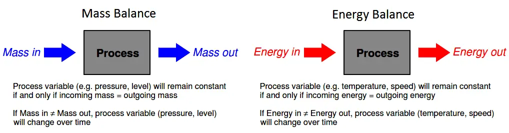
The example of an integrating process used here is just one of many possible processes where we are dealing with either a mass balance or an energy balance problem. “Mass balance” is the accounting of all mass into and out of a process. Since the Law of Mass Conservation states the impossibility of mass creation or destruction, all mass into and out of a process must be accounted for. If the mass flow rate into a process does not equal the mass flow rate out of a process, the process must be either gaining or losing an internal store of mass. The same may be said for energy: all energy flowing into and out of a process must be accounted for, since the Law of Energy Conservation states the impossibility of energy creation or destruction. If the energy flow rate (input power) into a process does not equal the energy flow rate (output power) out of a process, the process must be either gaining or losing an internal store of energy.
Common examples of integrating processes include the following:
• Liquid level control – mass balance – when the flow of liquid either into or out of a vessel is manipulated, and the other flows in or out of the vessel are constant
• Gas pressure control – mass balance – when the flow of gas either into or out of a vessel is manipulated, and the other flows in or out of the vessel are constant
• Storage bin level control – mass balance – when the conveyor feed rate into the bin is manipulated, and the draw from the bin is constant
• Temperature control – energy balance – when the flow of heat into or out of a process is manipulated, and all other heat flows are constant
• Speed control – energy balance – when the force (linear) or torque (angular) applied to a mass is manipulated, and all other loads are constant in force or torque
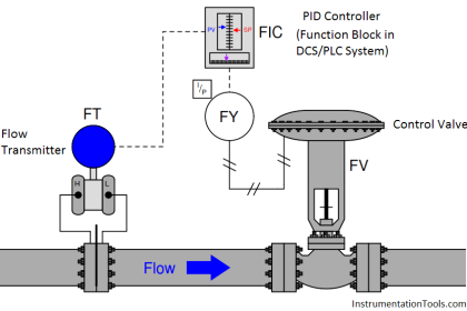
In a self-regulating process, the control element (valve) exerts control over both the in-flow and the out-flow of either mass or energy. In the previous subsection, where liquid flow control was the process example, the mass balance consisted of liquid flow into the valve and liquid flow out of the valve. Since the piping was essentially a “series” path for an incompressible fluid, where input flow must equal output flow at any given time, mass in and mass out were guaranteed to be in a state of balance, with one valve controlling both. This is why a change in valve position resulted in an almost immediate change and re-stabilization of flow rate: the valve exerts immediate control over both the incoming and the outgoing flow rates, with both in perfect balance. Therefore, nothing “integrates” over time in a liquid flow control process because there can never be an imbalance between in-flow and out-flow.
In an integrating process, the control element (valve) exerts control over either the in-flow or the out-flow of mass or energy, but never both. Thus, changing valve position in an integrating process causes an imbalance of mass flow and/or energy flow, resulting in the process variable ramping over time as either mass or energy accumulates in (or depletes from) the process.
Our “simple” example of an integrating (level-control) process becomes a bit more complicated if the outgoing flow depends on level, as is the case with a gravity-drained vessel where the outgoing flow is a function of liquid level in the vessel rather than being fixed at a constant rate as it was in the previous example:
If we subject the control valve to a manual step-change increase, the flow rate of liquid into the vessel immediately increases. This causes an imbalance of incoming and outgoing flow, resulting in the liquid level rising over time. As level rises, however, increasing hydrostatic pressure across the manual valve at the vessel outlet causes the outgoing flow rate to increase. This causes the mass imbalance rate to be less than it was before, resulting in a decreased integration rate (rate of level rise). Thus, the liquid level still rises, but at a slower and slower rate as time goes on. Eventually, the liquid level will become high enough that the pressure across the manual valve forces a flow rate out of the vessel equal to the flow rate into the vessel. At this point, with matched flow rates, the liquid level stabilizes with no corrective action from the controller (remember, the step-change in output was made in manual mode!). Note the final result of letting the outgoing flow be a function of liquid level: what used to be an integrating process has now become a self-regulating process, albeit one with a substantial lag time.
Many processes ideally categorized as integrating actually behave in this manner. Although the manipulated variable may control the flow rate into or out of a process, the other flow rates often change with the process variable. Returning to our list of integrating process examples, we see how a PV-variable load in each case can make the process self-regulate:
- Liquid level control – mass balance – if the in-flow naturally decreases as liquid level rises and/or the out-flow naturally increases as liquid level rises, the vessel’s liquid level will tend to self-regulate instead of integrate
- Gas pressure control – mass balance – if in-flow naturally decreases as pressure rises and/or the out-flow naturally increases as pressure rises, the vessel’s pressure will tend to self-regulate instead of integrate
- Storage bin level control – mass balance – if the draw from the bin increases with bin level (greater weight pushing material out at a faster rate), the bin’s level will tend to self-regulate instead of integrate
- Temperature control – energy balance – if the process naturally loses heat at a faster rate as temperature increases and/or the process naturally takes in less heat as temperature rises, the temperature will tend to self-regulate instead of integrate
- Speed control – energy balance – if drag forces on the object increase with speed (as they usually do for any fast-moving object), the speed will tend to self-regulate instead of integrate
We may generalize all these examples of integrating processes turned self-regulating by noting the one aspect common to all of them: some natural form of negative feedback exists internally to bring the system back into equilibrium. In the mass-balance examples, the physics of the process ensure a new balance point will eventually be reached because the in-flow(s) and/or out-flow(s) naturally change in ways that oppose any change in the process variable. In the energy-balance examples, the laws of physics again conspire to ensure a new equilibrium because the energy gains and/or losses naturally change in ways that oppose any change in the process variable. The presence of a control system is, of course, the ultimate example of negative feedback working to stabilize the process variable. However, the control system may not be the only form of negative feedback at work in a process. All self-regulating processes are that way because they intrinsically possess some degree of negative feedback acting as a sort of natural, proportional-only control system.
This one detail completely alters the fundamental characteristic of a process from integrating to self-regulating, and therefore changes the necessary controller parameters. Self-regulation guarantees at least some integral controller action is necessary to attain new setpoint values. A purely integrating process, by contrast, requires no integral controller action at all to achieve new setpoints, and in fact is guaranteed to suffer overshoot following setpoint changes if the controller is programmed with any integral action at all! Both types of processes, however, need some amount of integral action in the controller in order to recover from load changes.
Summary:
- Integrating processes are characterized by a ramping of the process variable in response to a step-change in the control element value or load(s).
- This integration occurs as a result of either mass flow imbalance or energy flow imbalance in and out of the process.
- Integrating processes are ideally controllable with proportional controller action alone.
- Integral controller action guarantees setpoint overshoot in a purely integrating process.
- Some integral controller action will be required in integrating processes to compensate for load changes.
- The amount of proportional controller action tolerable in an integrating process depends on the degree of time lag and process noise in the system. Too much proportional action will result in oscillation (time lags) and/or erratic control element motion (noise).
- An integrating process will become self-regulating if sufficient negative feedback is naturally introduced. This usually takes the form of loads varying with the process variable.