Process measurements reach the controller as a clean, straight line, but some measurements may need signal conversions. Some examples of nontrivial behavior are the differential-pressure flow signal, which depends on the square of the flow rate, and the stored volume in a horizontal tank, which changes nonlinearly with level. Given current automation technologies, the predictability of different processes is fundamental to ensure proper performance of the distributed control system (DCS).
Characterizer Blocks to Linearize Signals
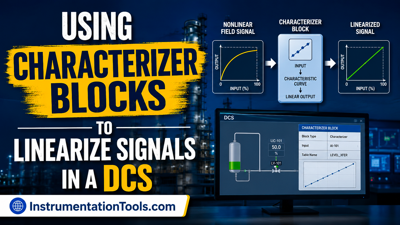
The basic DCS system is composed of a control loop, usually formed by a sensor and transmitter that measure the variable, a controller that compares the measurement against a setpoint, and a final control element, such as a valve, that acts on the process based on that comparison. A relevant component of the control loop is the software function block known as a proportional-integral-derivative (PID) controller.
The PID is responsible for calculating the so-called “error” value, which is the difference between a measured process variable (such as pressure, temperature, or flow) and a desired threshold. Before a PID controller can act on a signal predictably, the relationship between input and output often has to be straightened out. In a modern DCS, that task usually falls to a characterizer block.
A characterizer – also called a signal characterizer or function generator – converts one analog value into another according to a curve the engineer defines. The curve is not held as a formula, but as a short table of coordinate pairs. A block might store 10 or 20 (X, Y) points covering 0–100% of the input range. The block treats the function as a straight segment between any two adjacent breakpoints and computes intermediate outputs by linear interpolation.
Therefore, by taking a single segment bounded by points (x₁, y₁) and (x₂, y₂), the output for an input x is:
y = y₁ + (x − x₁) × (y₂ − y₁) / (x₂ − x₁)
This is the standard two-point interpolation formula, and you can reproduce any segment’s result using an online tool such as a linear interpolation calculator. There, you can enter the two breakpoints to find the correct interpolation function.
Square-root extraction for flow
The most common characterizer application is square-root extraction on orifice plates and other head-type flow measurements. The differential pressure across a restriction is proportional to the square of flow, so the transmitter output must be square-rooted to yield a signal that is linear in flow.
Many systems offer a dedicated square-root block, but the same result can be built with a characterizer whose breakpoints follow the square-root curve. Because that curve bends most sharply near zero, the breakpoints are spaced more closely at the low end, where a few widely spaced points would force the interpolation to cut across the true curve and introduce an error.
For example, consider a square-root characterizer in which breakpoints are chosen so that y = √x × 10, scaled to 0–100%. Two adjacent breakpoints are (9, 30) and (16, 40), which reflects the fact that 30% flow corresponds to 9% of the full differential pressure and 40% flow corresponds to 16%. For an input differential pressure (DP) of 12%, the block computes:
y = 30 + (12 − 9) × (40 − 30) / (16 − 9) ≈ 34.3%
By taking the true value at 12% DP, √12 × 10 ≈ 34.6%, you can see that the straight-segment fit undershoots the actual flow by about 0.3%. That residual gap is the consequence of approximating a curve with line segments, and it explains why the breakpoints near zero are placed closer together. At higher inputs, where the square-root function flattens, the same spacing produces a much smaller error. Running this check at every segment midpoint, against the formula y = √x × 10, is a routine way to confirm the configuration before the control loop is commissioned.
Linearizing an equal-percentage valve
The second common use is compensating for a control valve’s characteristic. A valve’s inherent characteristic describes the relationship between flow and travel under a constant pressure drop. Thus, the installed characteristic is what the loop actually sees, including line and equipment pressure losses. There are several online resources you can use to learn more about the differences among quick-opening, linear, and equal-percentage trims and how installed conditions shape them, such as this overview of valve characteristics.
An equal-percentage valve produces a small flow change near the seat and a large one near full open. If left uncorrected, this varies the loop gain across the operating range, making consistent tuning difficult. Consequently, a characterizer needs to be placed at the controller output to apply the approximate inverse of the installed characteristic, ensuring that equal increments of controller demand produce roughly equal increments of flow. The result is a loop gain that stays closer to constant, which is the condition PID tuning assumes.
Breakpoint count and interpolation error
Since the block interpolates linearly between points, the accuracy depends on how well the segments fit the underlying curve. It is worth noting that more breakpoints reduce the gap between the straight segments and the true function, but they also take longer to configure and verify.
The practical approach to solve this issue is to concentrate points where the curvature is highest and use fewer where the function is nearly straight. A useful check is to evaluate the function at the midpoint of each segment, compare the result with the true value, and add a breakpoint whenever the deviation exceeds the loop’s accuracy requirement.
The characterizer does not fix a bad measurement
Remember that a characterizer reshapes a signal, but it cannot recover information that was never measured correctly. If the input transmitter carries a zero shift, span shift, hysteresis, or linearity fault, those deviations can pass through the block and appear, reshaped, at its output. Therefore, it is crucial to characterize each of these instrumentation errors during calibration. The order of operations matters. So, you should calibrate and confirm the measurement first, then characterize it, since building a curve on top of an uncalibrated input only embeds the error in a less obvious form.
Characterizer blocks let a DCS convert nonlinear field signals into linear relationships that controllers and operators expect, using only a breakpoint table and linear interpolation between points. They are well-suited to square-root extraction and for compensating valve characteristics, provided the breakpoints are placed with the curve’s shape in mind and the upstream measurement is sound. Used in that order – accurate measurement, then characterization – they can be a great tool for removing a common source of inconsistent loop behavior without adding hardware.