Ziegler-Nichols open-loop tuning procedure
The next simulated process I attempted to tune was a liquid level-control process. Performing an open-loop test (one 10% increasing output step-change, followed by a 10% decreasing output step-change, both made in manual mode) on this process resulted in the following behavior:
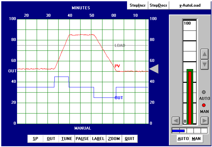
From the trend, the process appears to be purely integrating, as though the control valve were throttling the flow of liquid into a vessel with a constant out-flow. The reaction rate (R) on the first step-change is 50% over 10 minutes, or 5 percent per minute. Dead time (L) appears virtually nonexistent, estimated to be 0.1 minutes simply for the sake of having a dead-time value to use in the Ziegler-Nichols equations. Following the Ziegler-Nichols recommendations for PID tuning based on these process characteristics (also including the 10% step-change magnitude Δm):
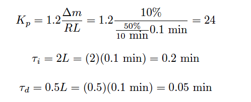
Applying the PID values of 24 (gain), 0.2 minutes per repeat (integral), and 0.05 minutes (derivative) gave the following result in automatic mode:
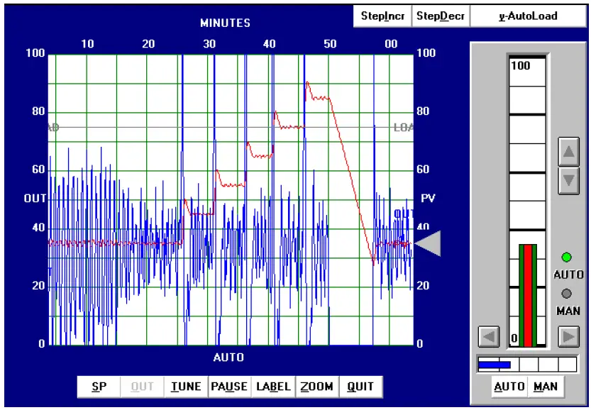
The process variable certainly responds rapidly to the five increasing setpoint changes and also to the one large decreasing setpoint change, but the valve action is hopelessly chaotic. Not only would this “jittery” valve motion prematurely wear out the stem packing, but it would also result in vast over-consumption of compressed air to continually stroke the valve from one extreme to the other. Furthermore, we see evidence of “overshoot” at every setpoint change, most likely from excessive integral action.
We can see from the valve’s wild behavior even during periods when the process variable is holding at setpoint that the problem is not a loop oscillation, but rather the effects of process noise on the controller. The extremely high gain value of 24 is amplifying PV noise by that factor, and reproducing it on the output signal.
Also Read : Ziegler-Nichols Open-Loop Theory
Ziegler-Nichols closed-loop tuning procedure
Next, I attempted to perform a closed-loop “Ultimate” gain test on this process, but I was not successful. Even the controller’s maximum possible gain value would not generate oscillations, due to the extremely crisp response of the process (minimal lag and dead times) and its integrating nature (constant phase shift of −90 o).
Heuristic tuning procedure
From the initial open-loop (manual output step-change) test, we could see this process was purely integrating. This told me it could be controlled primarily by proportional action, with very little integral action required, and no derivative action whatsoever. The presence of some process noise is the only factor limiting the aggressiveness of proportional action. With this in mind, I experimented with increasingly aggressive gain values until I reached a point where I felt the output signal noise was at a maximum acceptable limit for the control valve. Then, I experimented with integral action to ensure reasonable elimination of offset.
After some experimenting, the values I arrived at were 3 (gain), 10 minutes (integral), and 0 minutes (derivative). These tuning values represent a proportional action only one-eighth as aggressive as the Ziegler-Nichols recommendation, and an integral action fifty times less aggressive than the Ziegler-Nichols recommendation. The results of these tuning values in automatic mode are shown here:
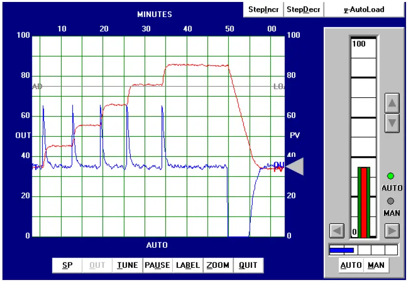
You can see on this trend five 10% increasing setpoint value changes, with crisp response every time, followed by a single 50% decreasing setpoint step-change. In all cases, the process response clearly meets the criteria of rapid attainment of new setpoint values and no overshoot or oscillation.
If it was decided that the noise in the output signal was too detrimental for the valve, we would have the option of further reducing the gain value and (possibly) compensating for slow offset recovery with more aggressive integral action. We could also attempt the insertion of a damping constant into either the level transmitter or the controller itself, so long as this added lag did not cause oscillation problems in the loop (Note). The best solution would be to find a way to isolate the level transmitter from noise, so that the process variable signal was much “quieter.” Whether or not this is possible depends on the process and on the particular transmitter used.
Note : We would have to be very careful with the addition of damping, since the oscillations could create may not appear on the trend. Remember that the insertion of damping (low-pass filtering) in the PV signal is essentially an act of “lying” to the controller: telling the controller something that differs from the real, measured signal. If our PV trend shows us this damped signal and not the “raw” signal from the transmitter, it is possible for the process to oscillate and the PV trend to be deceptively stable!
Also Read : Ziegler-Nichols Closed-Loop Theory