In reliability engineering, it is important to be able to quantity the reliability (or conversely, the probability of failure) for common components, and for systems comprised of those components.
As such, special terms and mathematical models have been developed to describe probability as it applies to component and system reliability.
Failure rate and MTBF of Safety Instrumented Systems
Perhaps the first and most fundamental measure of (un)reliability is the failure rate of a component or system of components, symbolized by the Greek letter lambda (λ).
The definition of “failure rate” for a group of components undergoing reliability tests is the instantaneous rate of failures per number of surviving components:
Where,
λ = Failure rate
Nf = Number of components failed during testing period
Ns = Number of components surviving during testing period
t = Time
The unit of measurement for failure rate (λ) is inverted time units (e.g. “per hour” or “per year”). An alternative expression for failure rate sometimes seen in reliability literature is the acronym FIT (“Failures In Time”), in units of 10−9 failures per hour.
Using a unit with a built-in multiplier such as 10−9 makes it easier for human beings to manage the very small λ values normally associated with high-reliability industrial components and systems.
Failure rate may also be applied to discrete-switching (on/off) components and systems of discrete-switching components on the basis of the number of on/off cycles rather than clock time. In such cases, we define failure rate in terms of cycles (c) instead of in terms of minutes, hours, or any other measure of time (t):
One of the conceptual difficulties inherent to the definition of lambda (λ) is that it is fundamentally a rate of failure over time. This is why the calculus notation dNf/dt is used to define lambda: a “derivative” in calculus always expresses a rate of change.
However, a failure rate is not the same thing as the number of devices failed in a test, nor is it the same thing as the probability of failure for one or more of those devices. Failure rate (λ) has more in common with the time constant of an resistor-capacitor circuit (τ ) than anything else.
An illustrative example is helpful here: if we were to test a large batch of identical components for proper operation over some extended period of time with no maintenance or other intervention, the number of failed components in that batch would gradually accumulate while the number of surviving components in the batch would gradually decline.
The reason for this is obvious: every component that fails remains failed (with no repair), leaving one fewer surviving component to function. If we limit the duration of this test to a time-span much shorter than the expected lifetime of the components, any failures that occur during the test must be due to random causes (“Acts of God”) rather than component wear-out.
This scenario is analogous to another random process: rolling a large set of dice, counting any “1” roll as a “fail” and any other rolled number as a “survive.” Imagine rolling the whole batch of dice at once, setting aside any dice landing on “1” aside (counting them as “failed” components in the batch), then only rolling the remaining dice the next time.
If we maintain this protocol – setting aside “failed” dice after each roll and only continuing to roll “surviving” dice the next time – we will find ourselves rolling fewer and fewer “surviving” dice in each successive roll of the batch.
Even though each of the six-sided die has a fixed failure probability of 1/6 , the population of “failed” dice keeps growing over time while the population of “surviving” dice keeps dwindling over time.
Not only does the number of surviving components in such a test dwindle over time, but that number dwindles at an ever-decreasing rate.
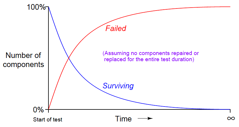
Likewise with the number of failures: the number of components failing (dice coming up “1”) is greatest at first, but then tapers off after the population of surviving components gets smaller and smaller. Plotted over time, the graph looks something like this:
Rapid changes in the failed and surviving component populations occurs at the start of the test when there is the greatest number of functioning components “in play.”
As components fail due to random events, the smaller and smaller number of surviving components results in a slower approach for both curves, simply because there are fewer surviving components remaining to fail.
These curves are precisely identical to those seen in RC (resistor-capacitor) charging circuits, with voltage and current tracing complementary paths: one climbing to 100% and the other falling to 0%, but both of them doing so at ever-decreasing rates.
Despite the asymptotic approach of both curves, however, we can describe their approaches in an RC circuit with a constant value τ , otherwise known as the time constant for the RC circuit. Failure rate (λ) plays a similar role in describing the failed/surviving curves of a batch of tested components:
Where,
Nsurviving = Number of components surviving at time t
Nfailed = Number of components failed at time t
No = Total number of components in test batch
e = Euler’s constant (≈ 2.71828)
λ = Failure rate (assumed to be a constant during the useful life period)
Following these formulae, we see that 63.2% of the components will fail (36.8% will survive) when λt = 1 (i.e. after one “time constant” has elapsed).
Unfortunately, this definition for lambda doesn’t make much intuitive sense. There is a way, however, to model failure rate in a way that not only makes more immediate sense, but is also more realistic to industrial applications.
Imagine a different testing protocol where we maintain a constant sample quantity of components over the entire testing period by immediately replacing each failed device with a working substitute as soon as it fails.
Now, the number of functioning devices under test will remain constant rather than declining as components fail. Imagine counting the number of “fails” (dice falling on a “1”) for each batch roll, and then rolling all the dice in each successive trial rather than setting aside the “failed” dice and only rolling those remaining.
If we did this, we would expect a constant fraction (1 /6) of the six-sided dice to “fail” with each and every roll. The number of failures per roll divided by the total number of dice would be the failure rate (lambda, λ) for these dice.
We do not see a curve over time because we do not let the failed components remain failed, and thus we see a constant number of failures with each period of time (with each group-roll).
We may mathematically express this using a different formula:
Where,
λ = Failure rate
Nf = Number of components failed during testing period
No = Number of components under test (maintained constant) during testing period by immediate replacement of failed components
t = Time
An alternative way of expressing the failure rate for a component or system is the reciprocal of lambda ( 1/λ ), otherwise known as Mean Time Between Failures (MTBF).
If the component or system in question is repairable, the expression Mean Time To Failure (MTTF) is often used instead. Whereas failure rate (λ) is measured in reciprocal units of time (e.g. “per hour” or “per year”), MTBF is simply expressed in units of time (e.g. “hours” or “years”).
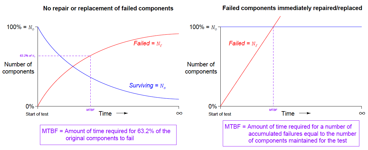
For non-maintained tests where the number of failed components accumulates over time (and the number of survivors dwindles), MTBF is precisely equivalent to “time constant” in an RC circuit: MTBF is the amount of time it will take for 63.2% of the components to fail due to random causes, leaving 36.8% of the component surviving.
For maintained tests where the number of functioning components remains constant due to swift repairs or replacement of failed components, MTBF (or MTTF) is the amount of time it will take for the total number of tested components to fail.
It should be noted that these definitions for lambda and MTBF are idealized, and do not necessarily represent all the complexity we see in real-life applications.
The task of calculating lambda or MTBF for any real component sample can be quite complex, involving statistical techniques well beyond the scope of instrument technician work.


