Imagine a liquid-level control system for a vessel, where the position of a level-sensing float directly sets the stem position of a control valve. As the liquid level rises, the valve opens up proportionally:
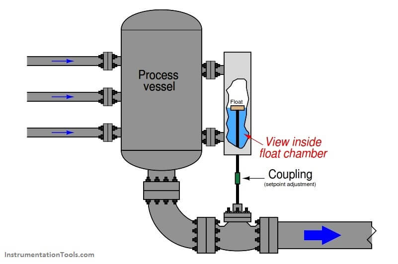
Despite its crude mechanical nature, this proportional control system would in fact help regulate the level of liquid inside the process vessel. If an operator wished to change the “setpoint” value of this level control system, he or she would have to adjust the coupling between the float and valve stems for more or less distance between the two. Increasing this distance (lengthening the connection) would effectively raise the level setpoint, while decreasing this distance (shortening the connection) would lower the setpoint.
We may generalize the proportional action of this mechanism to describe any form of controller where the output is a direct function of process variable (PV) and setpoint (SP):
m = Kpe + b
Where,
m = Controller output
e = Error (difference between PV and SP)
Kp = Proportional gain
b = Bias
A new term introduced with this formula is e, the “error” or difference between process variable and setpoint. Error may be calculated as SP−PV or as PV−SP, depending on whether or not the controller must produce an increasing output signal in response to an increase in the process variable (“direct” acting), or output a decreasing signal in response to an increase in the process variable (“reverse” acting):
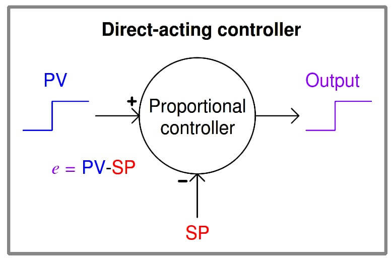
m = Kp (PV − SP) + b (Direct-acting proportional controller)
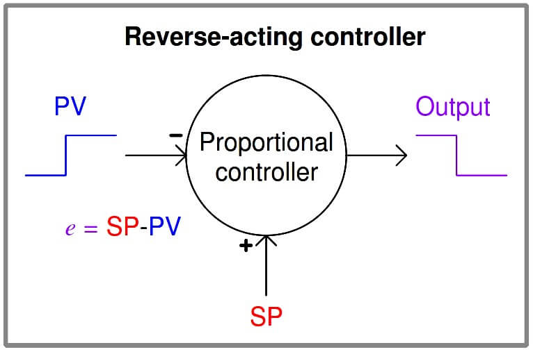
m = Kp (SP − PV) + b (Reverse-acting proportional controller)
The optional “+” and “−” symbols clarify the effect each input has on the controller output: a “−” symbol representing an inverting effect and a “+” symbol representing a noninverting effect. When we say that a controller is “direct-acting” or “reverse-acting” we are referring to it reaction to the PV signal, therefore the output signal from a “direct-acting” controller goes in the same direction as the PV signal and the output from a “reverse-acting” controller goes in the opposite direction of its PV signal.
It is important to note, however, that the response to a change in setpoint (SP) will yield the opposite response as does a change in process variable (PV): a rising SP will drive the output of a direct-acting controller down while a rising SP drives the output of a reverse-acting controller up. “+” and “−” symbols explicitly show the effect both inputs have on the controller output, helping to avoid confusion when analyzing the effects of PV changes versus the effects of SP changes.
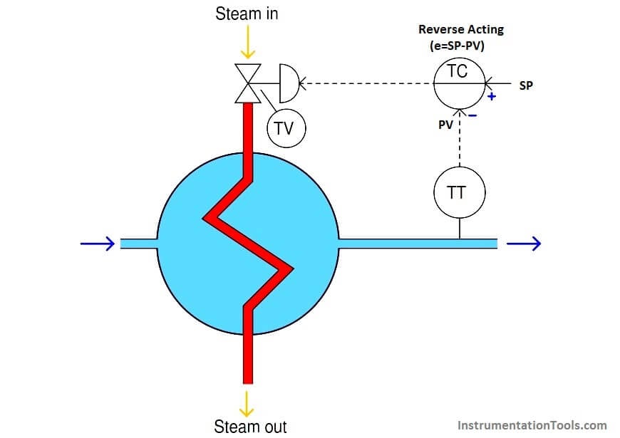
The direction of action required of the controller is determined by the nature of the process, transmitter, and final control element. In the case of the crude mechanical level controller, the action needs to be direct so that a greater liquid level will result in a further-open control valve to drain the vessel faster. In the case of the automated heat exchanger shown earlier, we are assuming that an increasing output signal sent to the control valve results in increased steam flow, and consequently higher temperature, so our controller will need to be reverse-acting (i.e. an increase in measured temperature results in a decrease in output signal; error calculated as SP−PV):
After the error has been calculated, the controller then multiplies the error signal by a constant value called the gain, which is programmed into the controller. The resulting figure, plus a “bias” quantity, becomes the output signal sent to the valve to proportion it. The “gain” value is exactly what it seems to be for anyone familiar with electronic amplifier circuits: a ratio of output to input. In this case, the gain of a proportional controller is the ratio of output signal change to input signal change, or how aggressive the controller reacts to changes in input (PV or SP).
To give a numerical example, a loop controller set to have a gain of 4 will change its output signal by 40% if it sees an input change of 10%: the ratio of output change to input change will be 4:1. Whether the input change comes in the form of a setpoint adjustment, a drift in the process variable, or some combination of the two does not matter to the magnitude of the output change.
The bias value of a proportional controller is simply the value of its output whenever process variable happens to be equal to setpoint (i.e. a condition of zero error ). Without a bias term in the proportional control formula, the valve would always return to a fully shut (0%) condition if ever the process variable reached the setpoint value. The bias term allows the final control element to achieve a non-zero state at setpoint.
If the controller could be configured for infinite gain, its response would duplicate on/off control. That is, any amount of error will result in the output signal becoming “saturated” at either 0% or 100%, and the final control element will simply turn on fully when the process variable drops below setpoint and turn off fully when the process variable rises above setpoint. Conversely, if the controller is set for zero gain, it will become completely unresponsive to changes in either process variable or setpoint: the valve will hold its position at the bias point no matter what happens to the process.
Obviously, then, we must set the gain somewhere between infinity and zero in order for this algorithm to function any better than on/off control. Just how much gain a controller needs to have depends on the process and all the other instruments in the control loop.
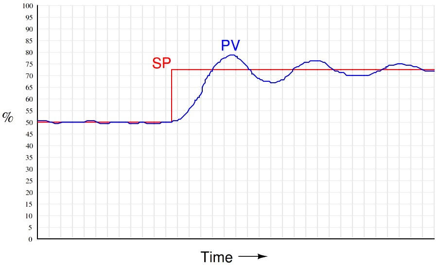
If the gain is set too high, there will be oscillations as the PV converges on a new setpoint value:
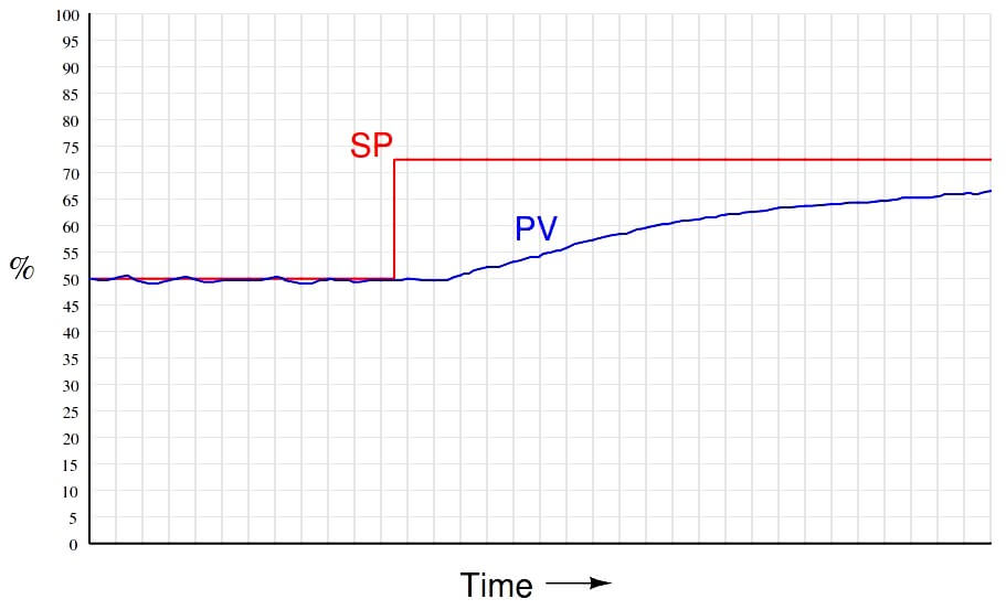
If the gain is set too low, the process response will be stable under steady-state conditions but relatively slow to respond to changes in setpoint, as shown in the following trend recording:
A characteristic deficiency of proportional control action, exacerbated with low controller gain values, is a phenomenon known as proportional-only offset where the PV never fully reaches SP. A full explanation of proportional-only offset is too lengthy for this discussion and will be presented in a subsequent article, but may be summarized here simply by drawing attention to the proportional controller equation which tells us the output always returns to the bias value when PV reaches SP (i.e. m = b when PV = SP). If anything changes in the process to require a different output value than the bias (b) to stabilize the PV, an error between PV and SP must develop to drive the controller output to that necessary output value. This means it is only by chance that the PV will settle precisely at the SP value – most of the time, the PV will deviate from SP in order to generate an output value sufficient to stabilize the PV and prevent it from drifting. This persistent error, or offset, worsens as the controller gain is reduced. Increasing controller gain causes this offset to decrease, but at the expense of oscillations.
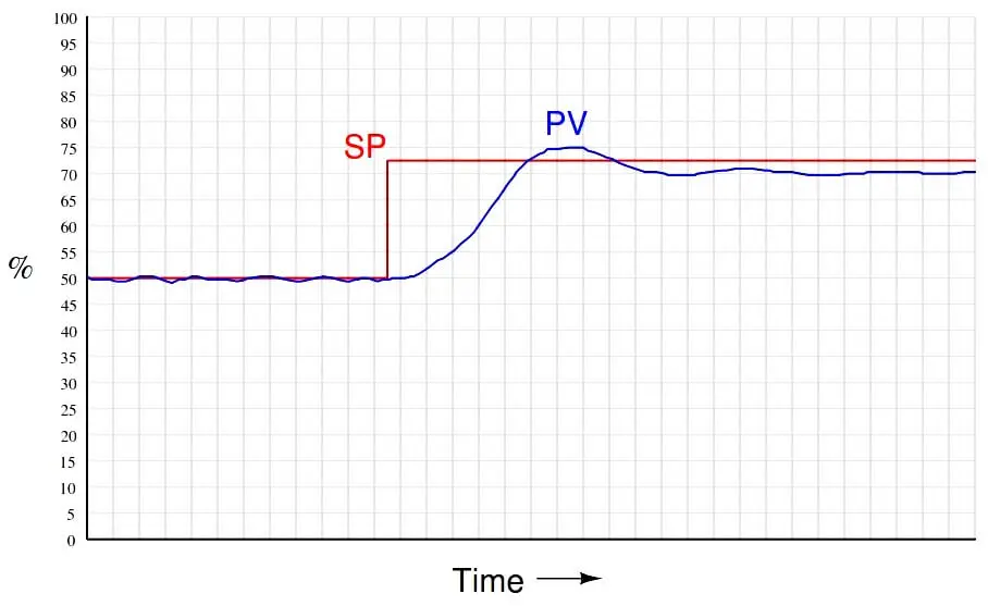
With proportional-only control, the choice of gain values is really a compromise between excessive oscillations and excessive offset. A well-tuned proportional controller response is shown here:
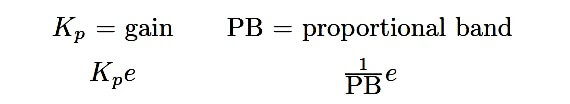
An unnecessarily confusing aspect of proportional control is the existence of two completely different ways to express controller proportionality. In the proportional-only equation shown earlier, the degree of proportional action was specified by the constant Kp , called gain. However, there is another way to express the sensitivity of proportional action, and that is to state the percentage of error change necessary to make the output (m) change by 100%. Mathematically, this is the inverse of gain, and it is called proportional band (PB):
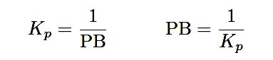
Gain is always specified as a unitless value , whereas proportional band is always specified as a percentage. For example, a gain value of 2.5 is equivalent to a proportional band value of 40%, because the error input to this controller must change by 40% in order to make the output change a full 100%.
Due to the existence of these two completely opposite conventions for specifying proportional action, you may see the proportional term of the control equation written differently depending on whether the author assumes the use of gain or the use of proportional band:
Many modern digital electronic controllers allow the user to conveniently select the unit they wish to use for proportional action. However, even with this ability, anyone tasked with adjusting a controller’s “tuning” values may be required to translate between gain and proportional band, especially if certain values are documented in a way that does not match the unit configured for the controller.
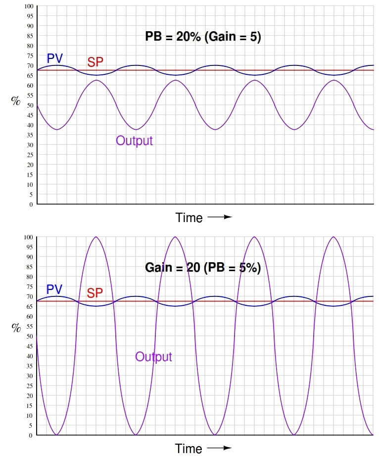
When you communicate the proportional action setting of a process controller, you should always be careful to specify either “gain” or “proportional band” to avoid ambiguity. Never simply say something like, “The proportional setting is twenty,” for this could mean either:
• Proportional band = 20%; Gain = 5 . . . or . . .
• Gain = 20; Proportional band = 5%
As you can see here, the real-life difference in controller response to an input disturbance (wave) depending on whether it has a proportional band of 20% or a gain of 20 is quite dramatic: