Through measurement, we try to obtain the value of an unknown parameter. However this measured value cannot be the actual or true value. If the measured value is very close to the true value, we call it to be a very accurate measuring system.
But before using the measured data for further use, one must have some idea how accurate is the measured data.
So error analysis is an integral part of measurement. We should also have clear idea what are the sources of error, how they can be reduced by properly designing the measurement methodology and also by repetitive measurements. These issues have been dwelt upon in this lesson.
Besides, for maintaining the accuracy the readings of the measuring instrument are frequently to be compared and adjusted with the reading of another standard instrument. This process is known as calibration.
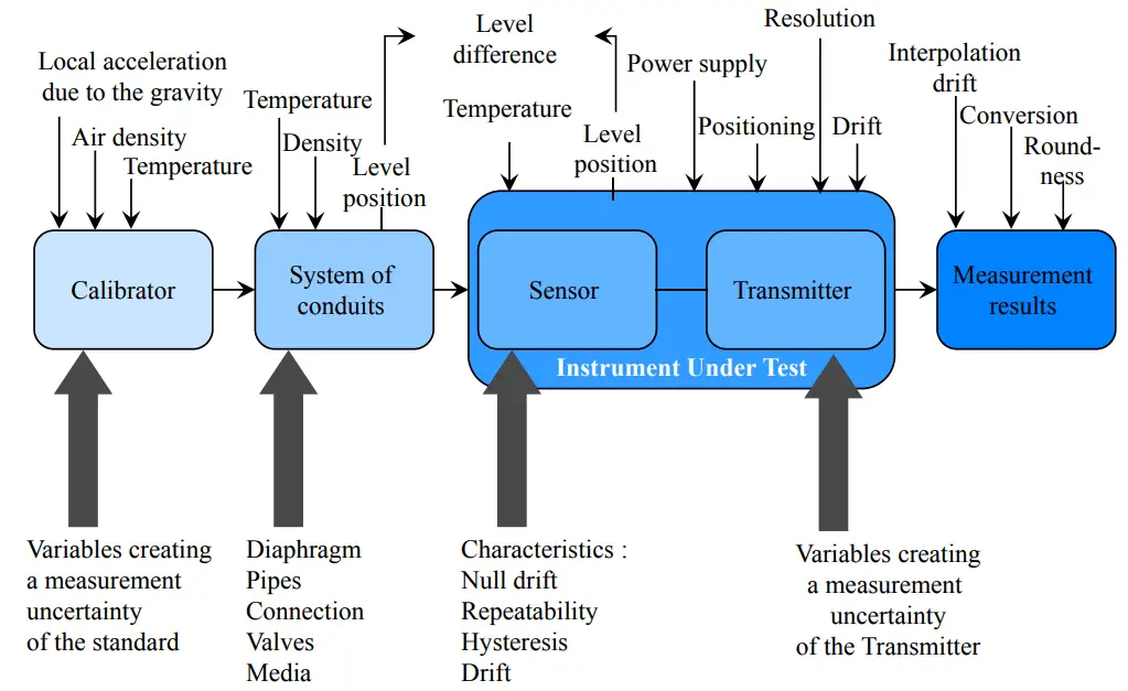
Image Courtesy : Endress + Hauser
Error Analysis
The term error in a measurement is defined as:
Error = Instrument reading – true reading.
Error is often expressed in percentage as:
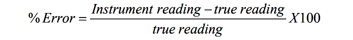
The errors in instrument readings may be classified in to three categories as:
- Gross errors
- Systematic errors
- Random Errors.
Gross errors arise due to human mistakes, such as, reading of the instrument value before it reaches steady state, mistake of recording the measured data in calculating a derived measured, etc. Parallax error in reading on an analog scale is also is also a source of gross error. Careful reading and recording of the data can reduce the gross errors to a great extent.
Systematic errors are those that affect all the readings in a particular fashion. Zero error, and bias of an instrument are examples of systematic errors. On the other hand, there are few errors, the cause of which is not clearly known, and they affect the readings in a random way. This type of errors is known as Random error. There is an important difference between the systematic errors and random errors. In most of the case, the systematic errors can be corrected by calibration, whereas the random errors can never be corrected, the can only be reduced by averaging, or error limits can be estimated.
Systematic errors may arise due to different reasons. It may be due to the shortcomings of the instrument or the sensor. An instrument may have a zero error, or its output may be varying in a nonlinear fashion with the input, thus deviating from the ideal linear input/output relationship. The amplifier inside the instrument may have input offset voltage and current which will contribute to zero error.
Different non-linearities in the amplifier circuit will also cause error due to nonlinearity. Besides, the systematic error can also be due to improper design of the measuring scheme. It may arise due to the loading effect, improper selection of the sensor or the filter cut off frequency. Systematic errors can be due to environmental effect also. The sensor characteristics may change with temperature or other environmental conditions.
The major feature of systematic errors is that the sources of errors are recognisable and can be reduced to a great extent by carefully designing the measuring system and selecting its components. By placing the instrument in a controlled environment may also help in reduction of systematic errors. They can be further reduced by proper and regular calibration of the instrument.
Random Errors : It has been already mentioned that the causes of random errors are not exactly known, so they cannot be eliminated. They can only be reduced and the error ranges can be estimated by using some statistical operations.
If we measure the same input variable a number of times, keeping all other factors affecting the measurement same, the same measured value would not be repeated, the consecutive reading would rather differ in a random way. But fortunately, the deviations of the readings normally follow a particular distribution (mostly normal distribution) and we may be able to reduce the error by taking a number of readings and averaging them out.
Calibration and Error reduction
It has already been mentioned that the random errors cannot be eliminated. But by taking a number of readings under the same condition and taking the mean, we can considerably reduce the random errors. In fact, if the number of readings is very large, we can say that the mean value will approach the true value, and thus the error can be made almost zero. For finite number of readings, by using the statistical method of analysis, we can also estimate the range of the measurement error.
On the other hand, the systematic errors are well defined, the source of error can be identified easily and once identified, it is possible to eliminate the systematic error. But even for a simple instrument, the systematic errors arise due to a number of causes and it is a tedious process to identify and eliminate all the sources of errors. An attractive alternative is to calibrate the instrument for different known inputs.
Calibration is a process where a known input signal or a series of input signals are applied to the measuring system. By comparing the actual input value with the output indication of the system, the overall effect of the systematic errors can be observed. The errors at those calibrating points are then made zero by trimming few adjustable components, by using calibration charts or by using software corrections.
Strictly speaking, calibration involves comparing the measured value with the standard instruments derived from comparison with the primary standards kept at Standard Laboratories. In an actual calibrating system for a pressure sensor (say), we not only require a standard pressure measuring device, but also a test-bench, where the desired pressure can be generated at different values.The calibration process of an acceleration measuring device is more difficult, since, the desired acceleration should be generated on a body, the measuring device has to be mounted on it and the actual value of the generated acceleration is measured in some indirect way.
The calibration can be done for all the points, and then for actual measurement, the true value can be obtained from a look-up table prepared and stored before hand. This type of calibration, is often referred as software calibration.
Alternatively, a more popular way is to calibrate the instrument at one, two or three points of measurement and trim the instrument through independent adjustments, so that, the error at those points would be zero. It is then expected that error for the whole range of measurement would remain within a small range. These types of calibration are known as single-point, two-point and three-point calibration. Typical input-output characteristics of a measuring device under these three calibrations are shown in below fig.
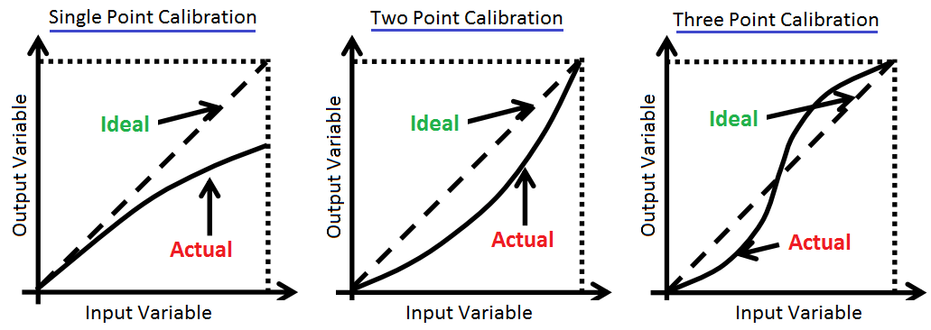
The single-point calibration is often referred as offset adjustment, where the output of the system is forced to be zero under zero input condition. For electronic instruments, often it is done automatically and is the process is known as auto-zero calibration. For most of the field instruments calibration is done at two points, one at zero input and the other at full scale input. Two independent adjustments, normally provided, are known as zero and span adjustments.
One important point needs to be mentioned at this juncture. The characteristics of an instrument change with time. So even it is calibrated once, the output may deviate from the calibrated points with time, temperature and other environmental conditions. So the calibration process has to be repeated at regular intervals if one wants that it should give accurate value of the measurand through out.
Conclusion
Errors and calibration are two major issues in measurement. In fact, knowledge on measurement remains incomplete without any comprehensive idea on these two issues.we discussed brief overview about errors and calibration. The terms error and limiting error have been defined and explained. The different types of error are also classified.
The methods for reducing random errors through repetitive measurements are explained. We have also discussed the least square straight line fitting technique. The propagation of error is also discussed. However, though the importance of mean and standard deviation has been elaborated, for the sake of brevity, the normal distribution, that random errors normally follows, has been left out. The performance of an instrument changes with time and many other physical parameters.
In order to ensure that the instrument reading will follow the actual value within reason accuracy, calibration is required at frequent intervals. In this process we compare and adjust the instrument readings to give true values at few selected readings. Different methods of calibration, e.g., single point calibration, two point calibration and three point calibration have been explained