The thermocouple is a simple, widely used component for measuring temperature.
Thermocouple Theory
A thermocouple, shown in Below Figure, consists of two wires of dissimilar metals joined together at one end, called the measurement (“hot”) junction. The other end, where the wires are not joined, is connected to the signal conditioning circuitry traces, typically made of copper. This junction between the thermocouple metals and the copper traces is called the reference (“cold”) junction.
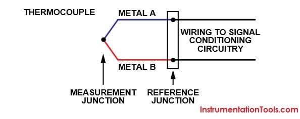
The voltage produced at the reference junction depends on the temperatures at both the measurement junction and the reference junction.
Since the thermocouple is a differential device rather than an absolute temperature measurement device, the reference junction temperature must be known to get an accurate absolute temperature reading. This process is known as reference junction compensation (cold junction compensation.)
Thermocouples have become the industry-standard method for cost-effective measurement of a wide range of temperatures with reasonable accuracy.
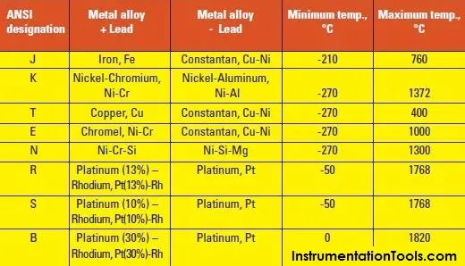
Thermocouple Types
Advantages of Thermocouples :
Temperature range: Most practical temperature ranges, from cryogenics to jet-engine exhaust, can be served using thermocouples. Depending on the metal wires used, a thermocouple is capable of measuring temperature in the range –200°C to +2500°C
Robust: Thermocouples are rugged devices that are immune to shock and vibration and are suitable for use in hazardous environments.
Rapid response: Because they are small and have low thermal capacity, thermocouples respond rapidly to temperature changes, especially if the sensing junction is exposed. They can respond to rapidly changing temperatures within a few hundred milliseconds.
No self heating: Because thermocouples require no excitation power, they are not prone to self heating and are intrinsically safe.
Disadvantages of Thermocouples :
Complex signal conditioning: Substantial signal conditioning is necessary to convert the thermocouple voltage into a usable temperature reading. Traditionally, signal conditioning has required a large investment in design time to avoid introducing errors that degrade accuracy.
Accuracy: In addition to the inherent inaccuracies in thermocouples due to their metallurgical properties, a thermocouple measurement is only as accurate as the reference junction temperature can be measured, traditionally within 1°C to 2°C.
Susceptibility to corrosion: Because thermocouples consist of two dissimilar metals, in some environments corrosion over time may result in deteriorating accuracy. Hence, they may need protection; and care and maintenance are essential.
Susceptibility to noise: When measuring microvolt-level signal changes, noise from stray electrical and magnetic fields can be a problem. Twisting the thermocouple wire pair can greatly reduce magnetic field pickup. Using a shielded cable or running wires in metal conduit and guarding can reduce electric field pickup. The measuring device should provide signal filtering, either in hardware or by software, with strong rejection of the line frequency (50 Hz/60 Hz) and its harmonics.
Difficulties in Measuring Temperature with Thermocouples
It is not easy to transform the voltage generated by a thermocouple into an accurate temperature reading for many reasons: the voltage signal is small, the temperature-voltage relationship is nonlinear, reference junction compensation is required, and thermocouples may pose grounding problems. Let’s consider these issues one by one.
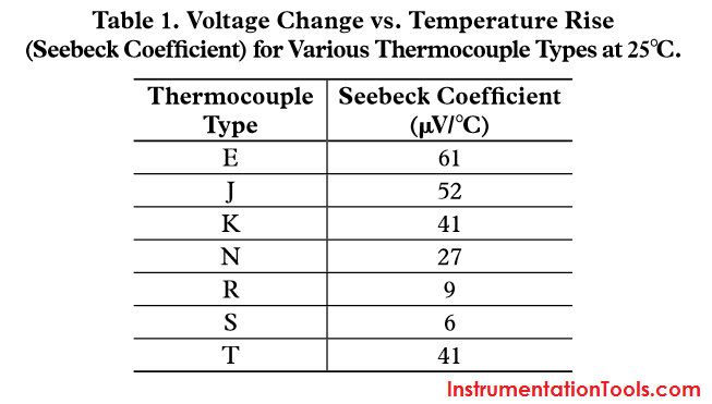
Voltage signal is small:
The most common thermocouple types are J, K, and T. At room temperature, their voltage varies at 52 μV/°C, 41μV/°C, and 41 μV/°C, respectively. Other less-common types have an even smaller voltage change with temperature.
This small signal requires a high gain stage before analog-to-digital conversion. Table 1 compares sensitivities of various thermocouple types.
Because the voltage signal is small, the signal-conditioning circuitry typically requires gains of about 100 or so—fairly straightforward signal conditioning.
What can be more difficult is distinguishing the actual signal from the noise picked up on the thermocouple leads. Thermocouple leads are long and often run through electrically noisy environments. The noise picked up on the leads can easily overwhelm the tiny thermocouple signal.
Two approaches are commonly combined to extract the signal from the noise. The first is to use a differential-input amplifier, such as an instrumentation amplifier, to amplify the signal. Because much of the noise appears on both wires (common-mode), measuring differentially eliminates it.
The second is low-pass filtering, which removes out-of-band noise. The low-pass filter should remove both radio-frequency interference (above 1 MHz) that may cause rectification in the amplifier and 50 Hz/60 Hz (power-supply) hum. It is important to place the filter for radio frequency interference ahead of the amplifier (or use an amplifier with filtered inputs).
The location of the 50-Hz/60-Hz filter is often not critical—it can be combined with the RFI filter, placed between the amplifier and ADC, incorporated as part of a sigma-delta ADC, or it can be programmed in software as an averaging filter.
Reference junction compensation:
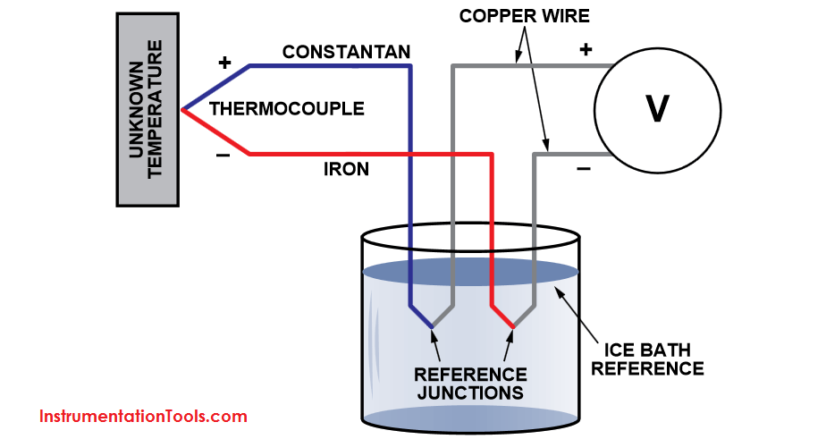
The temperature of the thermocouple’s reference junction must be known to get an accurate absolute-temperature reading. When thermocouples were first used, this was done by keeping the reference junction in an ice bath.
Below Figure depicts a thermocouple circuit with one end at an unknown temperature and the other end in an ice bath (0°C). This method was used to exhaustively characterize the various thermocouple types, thus almost all thermocouple tables use 0°C as the reference temperature.
But keeping the reference junction of the thermocouple in an ice bath is not practical for most measurement systems. Instead most systems use a technique called reference-junction compensation, (also known as cold-junction compensation).
The reference junction temperature is measured with another temperature-sensitive device—typically an IC, thermistor, diode, or RTD (resistance temperature-detector). The thermocouple voltage reading is then compensated to reflect the reference junction temperature.
It is important that the reference junction be read as accurately as possible—with an accurate temperature sensor kept at the same temperature as the reference junction. Any error in reading the reference junction temperature will show up directly in the final thermocouple reading.
A variety of sensors are available for measuring the reference temperature:
- Thermistors: They have fast response and a small package; but they require linearization and have limited accuracy, especially over a wide temperature range. They also require current for excitation, which can produce self-heating, leading to drift. Overall system accuracy, when combined with signal conditioning, can be poor.
- Resistance temperature-detectors (RTDs): RTDs are accurate, stable, and reasonably linear, however, package size and cost restrict their use to process-control applications.
- Remote thermal diodes: A diode is used to sense the temperature near the thermocouple connector. A conditioning chip converts the diode voltage, which is proportional to temperature, to an analog or digital output. Its accuracy is limited to about ±1°
- Integrated temperature sensor: An integrated temperature sensor, a standalone IC that senses the temperature locally, should be carefully mounted close to the reference junction, and can combine reference junction compensation and signal conditioning. Accuracies to within small fractions of 1°C can be achieved.
Voltage signal is nonlinear:
The slope of a thermocouple response curve changes over temperature. For example, at 0°C a T-type thermocouple output changes at 39 μV/°C, but at 100°C, the slope increases to 47 μV/°C.
There are three common ways to compensate for the nonlinearity of the thermocouple.
Choose a portion of the curve that is relatively flat and approximate the slope as linear in this region—an approach that works especially well for measurements over a limited temperature range.
No complicated computations are needed. One of the reasons the K- and J-type thermocouples are popular is that they both have large stretches of temperature for which the incremental slope of the sensitivity (Seebeck coefficient) remains fairly constant (see Below Figure).
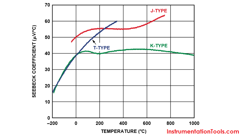
From Above Figure – Variation of thermocouple sensitivity with temperature. Note that K-type’s Seebeck coefficient is roughly constant at about 41 μV/°C from 0°C to 1000°C.
Another approach is to store in memory a lookup table that matches each of a set of thermocouple voltages to its respective temperature. Then use linear interpolation between the two closest points in the table to get other temperature values.
A third approach is to use higher order equations that model the behavior of the thermocouple. While this method is the most accurate, it is also the most computationally intensive. There are two sets of equations for each thermocouple. One set converts temperature to thermocouple voltage (useful for reference junction compensation). The other set converts thermocouple voltage to temperature.